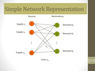
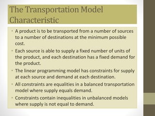
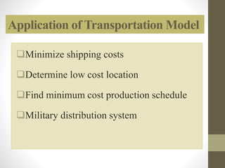
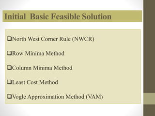
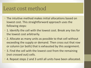
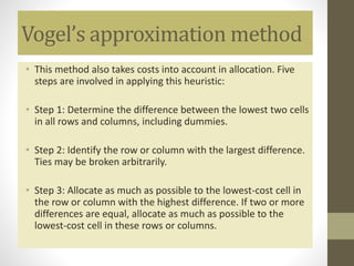
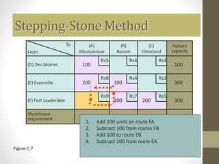
The transportation model aims to minimize shipping costs by finding the optimal distribution of goods from multiple sources to multiple destinations while satisfying supply and demand constraints. It encompasses both balanced and unbalanced transportation problems, with specialized methods such as the northwest corner rule and Vogel’s approximation method employed for obtaining initial and optimal solutions. The model is essential in various applications including cost minimization in logistics and production scheduling.

1. Transportation Model

2. Aim of Transportation Model
To find out optimum transportation
schedule keeping in mind cost of
transportation to be minimized.

3. What is a Transportation Problem?
• The transportation problem is a special type of
LPP where the objective is to minimize the cost
of distributing a product from a number of
sources or origins to a number of destinations.
• Because of its special structure the usual simplex
method is not suitable for solving transportation
problems. These problems require special
method of solution.

4. The Transportation Problem
• The problem of finding the minimum-cost
distribution of a given commodity
from a group of supply centers (sources) i=1,…,m
to a group of receiving centers (destinations)
j=1,…,n
• Each source has a certain supply (si)
• Each destination has a certain demand (dj)
• The cost of shipping from a source to a
destination is directly proportional to the
number of units shipped

5. Simple Network Representation
Transpor
tation-5
1
2
m
1
2
n
Sources Destinations
…
…
Supply s1
Supply s2
Supply sm
Demand d1
Demand d2
Demand dn
cij
Costs cij

6. The Transportation Model
Characteristic
• A product is to be transported from a number of sources
to a number of destinations at the minimum possible
cost.
• Each source is able to supply a fixed number of units of
the product, and each destination has a fixed demand for
the product.
• The linear programming model has constraints for supply
at each source and demand at each destination.
• All constraints are equalities in a balanced transportation
model where supply equals demand.
• Constraints contain inequalities in unbalanced models
where supply is not equal to demand.

7. Application of Transportation Model
Minimize shipping costs
Determine low cost location
Find minimum cost production schedule
Military distribution system

8. Two Types of Transportation
Problem
• Balanced Transportation Problem
where the total supply equals total demand
• Unbalanced Transportation Problem
where the total supply is not equal to the
total demand

9. Phases of Solution of
Transportation Problem
• Phase I- obtains the initial basic feasible
solution
• Phase II-obtains the optimal basic solution

10. Initial Basic Feasible Solution
North West Corner Rule (NWCR)
Row Minima Method
Column Minima Method
Least Cost Method
Vogle Approximation Method (VAM)

11. Northwest corner rule
• The northwest-corner rule requires that we start in
the upper left-hand cell (or northwest corner) of the
table and allocate units to shipping routes as follows:
• 1. Exhaust the supply (factory capacity) of each row
before moving down to the next row.
• 2. Exhaust the (warehouse) requirements of each
column before moving to the next column on the
right.
• 3. Check to ensure that all supplies and demands are
met.

12. Least cost method
• The intuitive method makes initial allocations based on
lowest cost. This straightforward approach uses the
following steps:
• 1. Identify the cell with the lowest cost. Break any ties for
the lowest cost arbitrarily.
• 2. Allocate as many units as possible to that cell without
exceeding the supply or demand. Then cross out that row
or column (or both) that is exhausted by this assignment.
• 3. Find the cell with the lowest cost from the remaining
(not crossed out) cells.
• 4. Repeat steps 2 and 3 until all units have been allocated.

13. Vogel’s approximation method
• This method also takes costs into account in allocation. Five
steps are involved in applying this heuristic:
• Step 1: Determine the difference between the lowest two cells
in all rows and columns, including dummies.
• Step 2: Identify the row or column with the largest difference.
Ties may be broken arbitrarily.
• Step 3: Allocate as much as possible to the lowest-cost cell in
the row or column with the highest difference. If two or more
differences are equal, allocate as much as possible to the
lowest-cost cell in these rows or columns.

14. Step 4: Stop the process if all row and column requirements
are met. If not, go to the next step.
Step 5: Recalculate the differences between the two lowest
cells remaining in all rows and columns. Any row and
column with zero supply or demand should not be used in
calculating further differences. Then go to Step 2.
The Vogel's approximation method (VAM) usually produces
an optimal or near- optimal starting solution. One study
found that VAM yields an optimum solution in 80 percent of
the sample problems tested.

15. Optimum Basic Solution
Stepping Stone Method
Modified Distribution Method a.k.a. MODI Method

16. Optimum Basic Solution:
Stepping-Stone Method
1. Select any unused square to evaluate
2. Beginning at this square, trace a closed
path back to the original square via
squares that are currently being used
3. Beginning with a plus (+) sign at the
unused corner, place alternate minus and
plus signs at each corner of the path just
traced

17. Stepping-Stone Method
4. Calculate an improvement index by first
adding the unit-cost figures found in each
square containing a plus sign and subtracting
the unit costs in each square containing a
minus sign
5. Repeat steps 1 though 4 until you have
calculated an improvement index for all
unused squares. If all indices are ≥ 0, you
have reached an optimal solution.

18. Problem Illustration
FROM
TO A.
ALBUQUERQU
E
B.
BOSTON
C.
CLEVELAND
FACTORY
CAPACITY
D. DES
MOINES 5 4 3 100
E. EVANSVILLE
8 4 3 300
F. FORT
LAUDERDALE 9 7 5 300
WAREHOUSE
DEMAND 300 200 200 700

19. Initial Feasible Solution using
Northwest Corner Rule
FROM
TO A.
ALBUQUERQU
E
B.
BOSTON
C.
CLEVELAND
FACTORY
CAPACITY
D. DES
MOINES 5 4
3
100
E. EVANSVILLE
8 4
3
300
F. FORT
LAUDERDALE 9 7
5
300
WAREHOUSE
DEMAND 300 200 200 700
100
200 100
100 200
IFS= DA + EA +EB + FB + FC = 100(5) + 200(8) + 100(4) + 100(7) + 200(5)
= 500 + 1600 + 400 + 700 + 1000 = 4200

20. Rs5
Rs8 Rs4
Rs4
+ -
+-
Optimizing Solution using
Stepping-Stone Method
To (A)
Albuquerque
(B)
Boston
(C)
Cleveland
(D) Des Moines
(E) Evansville
(F) Fort Lauderdale
Warehouse
requirement 300 200 200
Factory
capacity
300
300
100
700
Rs5
Rs5
Rs4
Rs4
Rs3
Rs3
$9
Rs8
$7
From
100
100
100
200
200
+-
-+
1
100
201 99
99
100200Figure C.5
Des Moines-
Boston index
= Rs4 – Rs5 + Rs8 - Rs4
= Rs3

21. Stepping-Stone Method
To (A)
Albuquerque
(B)
Boston
(C)
Cleveland
(D) Des Moines
(E) Evansville
(F) Fort Lauderdale
Warehouse
requirement 300 200 200
Factory
capacity
300
300
100
700
Rs5
Rs5
Rs4
Rs4
Rs3
Rs3
Rs9
Rs8
Rs7
From
100
100
100
200
200
Figure C.6
Start
+-
+
-+
-
Des Moines-Cleveland index
= Rs3 - Rs5 + Rs8 - Rs4 + Rs7 - Rs5 = Rs4

22. Stepping-Stone Method
To (A)
Albuquerque
(B)
Boston
(C)
Cleveland
(D) Des Moines
(E) Evansville
(F) Fort Lauderdale
Warehouse
requirement 300 200 200
Factory
capacity
300
300
100
700
Rs5
Rs5
Rs4
Rs4
Rs3
Rs3
Rs9
Rs8
Rs7
From
100
100
100
200
200
Evansville-Cleveland index
= Rs3 - Rs4 + Rs7 - Rs5 = Rs1
(Closed path = EC - EB + FB - FC)
Fort Lauderdale-Albuquerque index
= Rs9- Rs7 + Rs4 - Rs8 = -Rs1
(Closed path = FA - FB + EB - EA)

23. Stepping-Stone Method
1. If an improvement is possible, choose the
route (unused square) with the largest
negative improvement index
2. On the closed path for that route, select the
smallest number found in the squares
containing minus signs
3. Add this number to all squares on the closed
path with plus signs and subtract it from all
squares with a minus sign

24. Stepping-Stone Method
To (A)
Albuquerque
(B)
Boston
(C)
Cleveland
(D) Des Moines
(E) Evansville
(F) Fort Lauderdale
Warehouse
requirement 300 200 200
Factory
capacity
300
300
100
700
Rs5
Rs5
Rs4
Rs4
Rs3
Rs3
Rs9
Rs8
Rs7
From
100
100
100
200
200
Figure C.7
+
+-
-
1. Add 100 units on route FA
2. Subtract 100 from routes FB
3. Add 100 to route EB
4. Subtract 100 from route EA

25. Stepping-Stone Method
To (A)
Albuquerque
(B)
Boston
(C)
Cleveland
(D) Des Moines
(E) Evansville
(F) Fort Lauderdale
Warehouse
requirement 300 200 200
Factory
capacity
300
300
100
700
Rs5
Rs5
Rs4
Rs4
Rs3
Rs3
Rs9
Rs8
Rs7
From
100
200
100
100
200
Figure C.8
Total Cost = Rs5(100) + Rs8(100) + Rs4(200) + Rs9(100) + Rs5(200)
= Rs4,000

26. Special Issues in Modeling
 Demand not equal to supply
 Called an unbalanced problem
 Common situation in the real world
 Resolved by introducing dummy
sources or dummy destinations as
necessary with cost coefficients of zero

27. Special Issues in Modeling
Figure C.9
New
Des Moines
capacity
To (A)
Albuquerque
(B)
Boston
(C)
Cleveland
(D) Des Moines
(E) Evansville
(F) Fort Lauderdale
Warehouse
requirement 300 200 200
Factory
capacity
300
300
250
850
Rs5
Rs5
Rs4
Rs4
Rs3
Rs3
Rs9
Rs8
Rs7
From
50200
250
50
150
Dummy
150
0
0
0
150
Total Cost = 250(Rs5) + 50(Rs8) + 200(Rs4) + 50(Rs3) + 150(Rs5) + 150(0)
= Rs3,350

28. Special Issues in Modeling
 Degeneracy
 To use the stepping-stone methodology,
the number of occupied squares in any
solution must be equal to the number of
rows in the table plus the number of
columns minus 1
 If a solution does not satisfy this rule it is
called degenerate

29. To Customer
1
Customer
2
Customer
3
Warehouse 1
Warehouse 2
Warehouse 3
Customer
demand 100 100 100
Warehouse
supply
120
80
100
300
Rs8
Rs7
Rs2
Rs9
Rs6
Rs9
Rs7
Rs10
Rs10
From
Special Issues in Modeling
0 100
100
80
20
Figure C.10
Initial solution is degenerate
Place a zero quantity in an unused square and
proceed computing improvement indices

30. Thank you