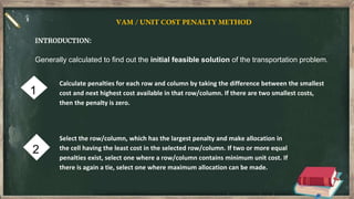
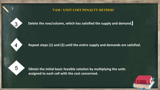
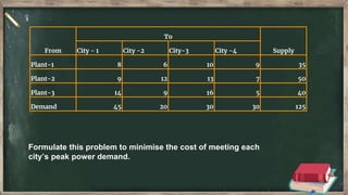
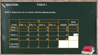
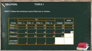
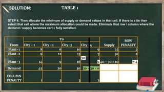
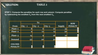
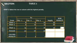
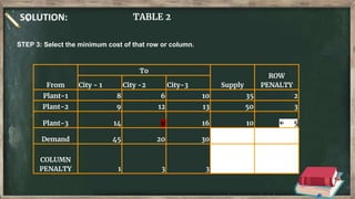
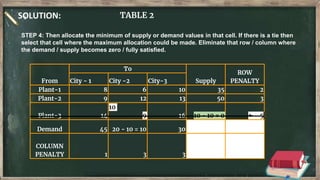
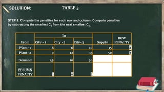
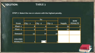
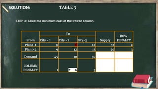
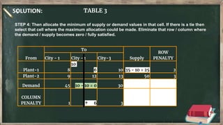
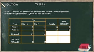
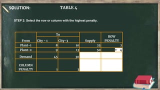
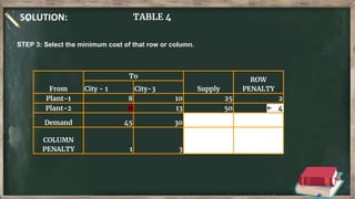
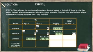
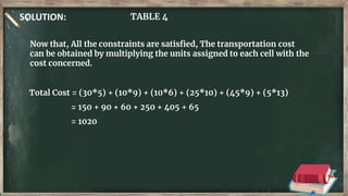
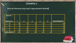
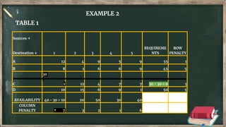
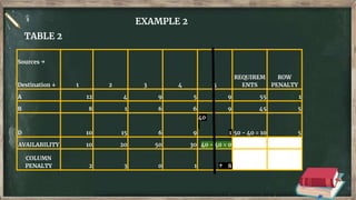
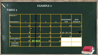
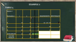
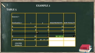
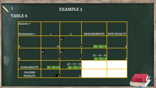
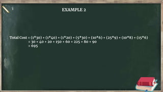
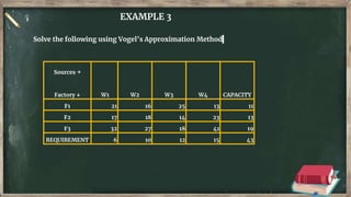
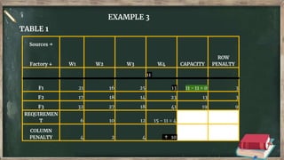
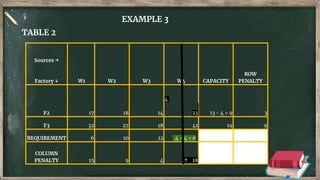
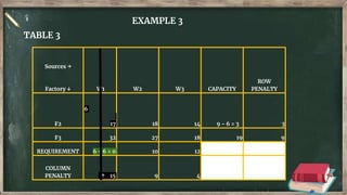
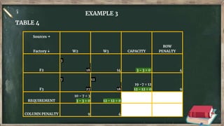
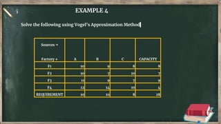
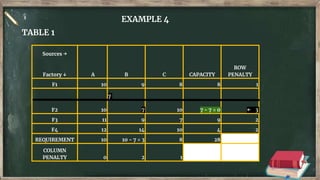
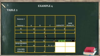
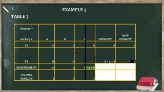
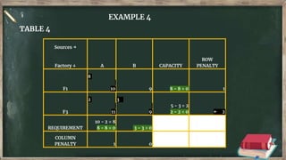
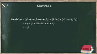
ETHIRAJ COLLEGE FOR WOMEN (Autonomous)
Chennai – 600 008
Prepared by
Ms.Swetha Shree R M.A.,M.Phil.
Department of Business Economics
Topic: Vogel’s Approximation Method
VOGEL’S APPROXIMATION METHOD
(VAM)
1
2
VAM / UNIT COST PENALTY METHOD
INTRODUCTION:
Generally calculated to find out the initial feasible solution of the transportation problem.
Calculate penalties for each row and column by taking the difference between the smallest
cost and next highest cost available in that row/column. If there are two smallest costs,
then the penalty is zero.
Select the row/column, which has the largest penalty and make allocation in
the cell having the least cost in the selected row/column. If two or more equal
penalties exist, select one where a row/column contains minimum unit cost. If
there is again a tie, select one where maximum allocation can be made.
3
5
VAM / UNIT COST PENALTY METHOD
Delete the row/column, which has satisfied the supply and demand.
Obtain the initial basic feasible solution by multiplying the units
assigned to each cell with the cost concerned.
4 Repeat steps (1) and (2) until the entire supply and demands are satisfied.
EXAMPLE 1
Consider the following example : Adani Power Limited which is an electric power
producing company in India Three electric power plants that supply the needs of
4 cities. each power plant can supply the following number of kilowatt hours off
electricity: Plant 1- 35 million; plant 2 - 50 million; plant 3 - 40 million.
The peak power demands in these cities which occur at the same time are as
follows : City 1 -45 million; City 2 - 20 million; City 3-30 million; City 4 - 30 million.
The cost of sending 1 million kilowatt hour of electricity from plant to city
depends on the distance the electricity must travel. Consider the following table
Formulate this problem to minimise the cost of meeting each
city’s peak power demand.
From
To
Supply
City - 1 City -2 City-3 City -4
Plant-1 8 6 10 9 35
Plant-2 9 12 13 7 50
Plant-3 14 9 16 5 40
Demand 45 20 30 30 125
SOLUTION: TABLE 1
From
To
Supply
ROW
PENALTY
City - 1 City -2 City-3 City -4
Plant-1 8 6 10 9 35 2
Plant-2 9 12 13 7 50 2
Plant-3 14 9 16 5 40 4
Demand 45 20 30 30 125
COLUMN
PENALTY 1 3 3 2
STEP 1: Compute the penalties for each row and column: Compute penalties
by subtracting the smallest Cij from the next smallest Cij ,
SOLUTION: TABLE 1
From
To
Supply
ROW
PENALTY
City - 1 City -2 City-3 City -4
Plant-1 8 6 10 9 35 2
Plant-2 9 12 13 7 50 2
Plant-3 14 9 16 5 40 ← 4
Demand 45 20 30 30 125
COLUMN
PENALTY 1 3 3 2
STEP 2: Select the row or column with the highest penalty.
SOLUTION: TABLE 1
From
To
Supply
ROW
PENALTY
City - 1 City -2 City-3 City -4
Plant-1 8 6 10 9 35 2
Plant-2 9 12 13 7 50 2
Plant-3 14 9 16 5 40 ← 4
Demand 45 20 30 30 125
COLUMN
PENALTY 1 3 3 2
STEP 3: Select the minimum cost of that row or column.
SOLUTION: TABLE 1
From
To
Supply
ROW
PENALTY
City - 1 City -2 City-3 City -4
Plant-1 8 6 10 9 35 2
Plant-2 9 12 13 7 50 2
Plant-3 14 9 16
30
5 40 - 30 = 10 ← 4
Demand 45 20 30 30 - 30 = 0
COLUMN
PENALTY 1 3 3 2
STEP 4: Then allocate the minimum of supply or demand values in that cell. If there is a tie then
select that cell where the maximum allocation could be made. Eliminate that row / column where the
demand / supply becomes zero / fully satisfied.
SOLUTION: TABLE 1
STEP 5: Continue until all constraints are satisfied.
SOLUTION: TABLE 2
From
To
Supply
ROW
PENALTY
City - 1 City -2 City-3
Plant-1 8 6 10 35 2
Plant-2 9 12 13 50 3
Plant-3 14 9 16 10 5
Demand 45 20 30
COLUMN
PENALTY 1 3 3
STEP 1: Compute the penalties for each row and column: Compute penalties
by subtracting the smallest Cij from the next smallest Cij ,
SOLUTION: TABLE 2
From
To
Supply
ROW
PENALTY
City - 1 City -2 City-3
Plant-1 8 6 10 35 2
Plant-2 9 12 13 50 3
Plant-3 14 9 16 10 ← 5
Demand 45 20 30
COLUMN
PENALTY 1 3 3
STEP 2: Select the row or column with the highest penalty.
SOLUTION: TABLE 2
From
To
Supply
ROW
PENALTY
City - 1 City -2 City-3
Plant-1 8 6 10 35 2
Plant-2 9 12 13 50 3
Plant-3 14 9 16 10 ← 5
Demand 45 20 30
COLUMN
PENALTY 1 3 3
STEP 3: Select the minimum cost of that row or column.
SOLUTION: TABLE 2
From
To
Supply
ROW
PENALTY
City - 1 City -2 City-3
Plant-1 8 6 10 35 2
Plant-2 9 12 13 50 3
Plant-3 14
10
9 16 10 - 10 = 0 ← 5
Demand 45 20 - 10 = 10 30
COLUMN
PENALTY 1 3 3
STEP 4: Then allocate the minimum of supply or demand values in that cell. If there is a tie then
select that cell where the maximum allocation could be made. Eliminate that row / column where
the demand / supply becomes zero / fully satisfied.
SOLUTION: TABLE 2
STEP 5: Continue until all constraints are satisfied.
SOLUTION: TABLE 3
From
To
Supply
ROW
PENALTY
City - 1 City -2 City-3
Plant-1 8 6 10 35 2
Plant-2 9 12 13 50 3
Demand 45 10 30
COLUMN
PENALTY 1 6 3
STEP 1: Compute the penalties for each row and column: Compute penalties
by subtracting the smallest Cij from the next smallest Cij ,
SOLUTION: TABLE 3
From
To
Supply
ROW
PENALTY
City - 1 City -2 City-3
Plant-1 8 6 10 35 2
Plant-2 9 12 13 50 3
Demand 45 10 30
COLUMN
PENALTY 1 ↑ 6 3
STEP 2: Select the row or column with the highest penalty.
SOLUTION: TABLE 3
From
To
Supply
ROW
PENALTY
City - 1 City -2 City-3
Plant-1 8 6 10 35 2
Plant-2 9 12 13 50 3
Demand 45 10 30
COLUMN
PENALTY 1 ↑ 6 3
STEP 3: Select the minimum cost of that row or column.
SOLUTION: TABLE 3
From
To
Supply
ROW
PENALTY
City - 1 City -2 City-3
Plant-1 8
10
6 10 35 - 10 = 25 2
Plant-2 9 12 13 50 3
Demand 45 10 - 10 = 0 30
COLUMN
PENALTY 1 ↑ 6 3
STEP 4: Then allocate the minimum of supply or demand values in that cell. If there is a tie then
select that cell where the maximum allocation could be made. Eliminate that row / column where
the demand / supply becomes zero / fully satisfied.
SOLUTION: TABLE 3
STEP 5: Continue until all constraints are satisfied.
SOLUTION: TABLE 4
From
To
Supply
ROW
PENALTY
City - 1 City-3
Plant-1 8 10 25 2
Plant-2 9 13 50 4
Demand 45 30
COLUMN
PENALTY 1 3
STEP 1: Compute the penalties for each row and column: Compute penalties
by subtracting the smallest Cij from the next smallest Cij ,
SOLUTION: TABLE 4
From
To
Supply
ROW
PENALTY
City - 1 City-3
Plant-1 8 10 25 2
Plant-2 9 13 50 ← 4
Demand 45 30
COLUMN
PENALTY 1 3
STEP 2: Select the row or column with the highest penalty.
SOLUTION: TABLE 4
From
To
Supply
ROW
PENALTY
City - 1 City-3
Plant-1 8 10 25 2
Plant-2 9 13 50 ← 4
Demand 45 30
COLUMN
PENALTY 1 3
STEP 3: Select the minimum cost of that row or column.
SOLUTION: TABLE 4
From
To
Supply
ROW
PENALTY
City - 1 City-3
Plant-1 8
25
10 25 - 25 = 0 2
Plant-2
45
9
5
13
50 - 45 = 5
5 - 5 = 0 ← 4
Demand 45 - 45 = 0
30 - 5 = 25
25 - 25 = 0
COLUMN
PENALTY 1 3
STEP 4: Then allocate the minimum of supply or demand values in that cell. If there is a tie then
select that cell where the maximum allocation could be made. Eliminate that row / column where
the demand / supply becomes zero / fully satisfied.
SOLUTION: TABLE 4
Now that, All the constraints are satisfied, The transportation cost
can be obtained by multiplying the units assigned to each cell with the
cost concerned.
Total Cost = (30*5) + (10*9) + (10*6) + (25*10) + (45*9) + (5*13)
= 150 + 90 + 60 + 250 + 405 + 65
= 1020
EXAMPLE 2
Solve the following using Vogel’s Approximation Method
Sources →
Destination ↓ 1 2 3 4 5 REQUIREMENTS
A 12 4 9 5 9 55
B 8 1 6 6 9 45
C 1 12 4 7 7 30
D 10 15 6 9 1 50
AVAILABILITY 40 20 50 30 40 180
EXAMPLE 2
TABLE 1
Sources →
Destination ↓ 1 2 3 4 5
REQUIREME
NTS
ROW
PENALTY
A 12 4 9 5 9 55 1
B 8 1 6 6 9 45 5
C
30
1 12 4 7 7 30 - 30 = 0 3
D 10 15 6 9 1 50 5
AVAILABILITY 40 - 30 = 10 20 50 30 40
COLUMN
PENALTY ↑ 7 3 2 1 6
EXAMPLE 2
TABLE 2
Sources →
Destination ↓ 1 2 3 4 5
REQUIREM
ENTS
ROW
PENALTY
A 12 4 9 5 9 55 1
B 8 1 6 6 9 45 5
D 10 15 6 9
40
1 50 - 40 = 10 5
AVAILABILITY 10 20 50 30 40 - 40 = 0
COLUMN
PENALTY 2 3 0 1 ↑ 8
EXAMPLE 2
TABLE 3
Sources →
Destination ↓ 1 2 3 4
REQUIREME
NTS
ROW
PENALTY
A 12 4 9 5 55 1
B 8
20
1 6 6 45 - 20 = 25 ← 5
D 10 15 6 9 10 3
AVAILABILIT
Y 10 20 - 20 = 0 50 30
COLUMN
PENALTY 2 3 0 1
EXAMPLE 2
TABLE 4
Sources →
Destination ↓ 1 3 4 REQUIREMENTS ROW PENALTY
A 12 9
30
5 55 - 30 = 25 ← 4
B 8 6 6 25 0
D 10 6 9 10 3
AVAILABILITY 10 50 30 - 30 = 0
COLUMN
PENALTY 2 0 1
EXAMPLE 2
TABLE 5
Sources →
Destination ↓ 1 3 REQUIREMENTS ROW PENALTY
A 12 9 25 3
B 8 6 25 2
D 10
10
6 10 - 10 = 0 ← 4
AVAILABILITY 10 50 - 10 = 40
COLUMN
PENALTY 2 0
EXAMPLE 2
TABLE 6
Sources →
Destination ↓ 1 3 REQUIREMENTS ROW PENALTY
A 12
25
9 25 - 25 = 0 3
B
10
8
15
6
25 - 10 = 15
15 - 15 = 0 2
AVAILABILITY 10 - 10 = 0
40 - 15 = 25
25 - 25 = 0
COLUMN
PENALTY ↑ 4 3
EXAMPLE 2
Total Cost = (1*30) + (1*40) + (1*20) + (5*30) + (10*6) + (25*9) + (10*8) + (15*6)
= 30 + 40 + 20 + 150 + 60 + 225 + 80 + 90
= 695
EXAMPLE 3
Solve the following using Vogel’s Approximation Method
Sources →
Factory ↓ W1 W2 W3 W4 CAPACITY
F1 21 16 25 13 11
F2 17 18 14 23 13
F3 32 27 18 41 19
REQUIREMENT 6 10 12 15 43
EXAMPLE 3
TABLE 1
Sources →
Factory ↓ W1 W2 W3 W4 CAPACITY
ROW
PENALTY
F1 21 16 25
11
13 11 - 11 = 0 3
F2 17 18 14 23 13 3
F3 32 27 18 41 19 9
REQUIREMEN
T 6 10 12 15 - 11 = 4
COLUMN
PENALTY 4 2 4 ↑ 10
EXAMPLE 3
TABLE 2
Sources →
Factory ↓ W1 W2 W3 W4 CAPACITY
ROW
PENALTY
F2 17 18 14
4
23 13 - 4 = 9 3
F3 32 27 18 41 19 9
REQUIREMENT 6 10 12 4 - 4 = 0
COLUMN
PENALTY 15 9 4 ↑ 18
EXAMPLE 3
TABLE 3
Sources →
Factory ↓ W1 W2 W3 CAPACITY
ROW
PENALTY
F2
6
17 18 14 9 - 6 = 3 3
F3 32 27 18 19 9
REQUIREMENT 6 - 6 = 0 10 12
COLUMN
PENALTY ↑ 15 9 4
EXAMPLE 3
TABLE 4
Sources →
Factory ↓ W2 W3 CAPACITY
ROW
PENALTY
F2
3
18 14 3 - 3 = 0 4
F3
7
27
12
18
19 -7 = 12
12 - 12 = 0 9
REQUIREMENT
10 - 7 = 3
3 - 3 = 0 12 - 12 = 0
COLUMN PENALTY 9 4
EXAMPLE 3
Total Cost = (11*13) + (4*23) + (6*17) + (3*18) + (7*27) + (12*18)
= 143 + 92 + 102 + 54 + 189 + 216
= 796
EXAMPLE 4
Solve the following using Vogel’s Approximation Method
Sources →
Factory ↓ A B C CAPACITY
F1 10 9 8 8
F2 10 7 10 7
F3 11 9 7 9
F4 12 14 10 4
REQUIREMENT 10 10 8 28
EXAMPLE 4
TABLE 1
Sources →
Factory ↓ A B C CAPACITY
ROW
PENALTY
F1 10 9 8 8 1
F2 10
7
7 10 7 - 7 = 0 ← 3
F3 11 9 7 9 2
F4 12 14 10 4 2
REQUIREMENT 10 10 - 7 = 3 8 28
COLUMN
PENALTY 0 2 1
EXAMPLE 4
TABLE 2
Sources →
Factory ↓ A B C CAPACITY
ROW
PENALTY
F1 10 9 8 8 1
F3 11 9 7 9 2
F4 12 14
4
10 4 - 4 = 0 ← 2
REQUIREMEN
T 10 3 8 - 4 = 4
COLUMN
PENALTY 1 0 1
EXAMPLE 4
TABLE 3
Sources →
Factory ↓ A B C CAPACITY
ROW
PENALTY
F1 10 9 8 8 1
F3 11 9
4
7 9 - 4 = 5 ← 2
REQUIREMENT 10 3 4 - 4 = 0
COLUMN
PENALTY 1 0 1
EXAMPLE 4
TABLE 4
Sources →
Factory ↓ A B CAPACITY
ROW
PENALTY
F1
8
10 9 8 - 8 = 0 1
F3
2
11
3
9
5 - 3 = 2
2 - 2 = 0 ← 2
REQUIREMENT
10 - 2 = 8
8 - 8 = 0 3 - 3 = 0
COLUMN
PENALTY 1 0
EXAMPLE 4
Total Cost = (7*7) + (4*10) + (4*7) + (8*10) + (2*11) + (3*9)
= 49 + 40 + 28 + 80 + 22 + 27
= 246
THANK YOU

VOGEL'S APPROXIMATION METHOD

  • 1.
    ETHIRAJ COLLEGE FORWOMEN (Autonomous) Chennai – 600 008 Prepared by Ms.Swetha Shree R M.A.,M.Phil. Department of Business Economics Topic: Vogel’s Approximation Method
  • 2.
  • 3.
    1 2 VAM / UNITCOST PENALTY METHOD INTRODUCTION: Generally calculated to find out the initial feasible solution of the transportation problem. Calculate penalties for each row and column by taking the difference between the smallest cost and next highest cost available in that row/column. If there are two smallest costs, then the penalty is zero. Select the row/column, which has the largest penalty and make allocation in the cell having the least cost in the selected row/column. If two or more equal penalties exist, select one where a row/column contains minimum unit cost. If there is again a tie, select one where maximum allocation can be made.
  • 4.
    3 5 VAM / UNITCOST PENALTY METHOD Delete the row/column, which has satisfied the supply and demand. Obtain the initial basic feasible solution by multiplying the units assigned to each cell with the cost concerned. 4 Repeat steps (1) and (2) until the entire supply and demands are satisfied.
  • 5.
    EXAMPLE 1 Consider thefollowing example : Adani Power Limited which is an electric power producing company in India Three electric power plants that supply the needs of 4 cities. each power plant can supply the following number of kilowatt hours off electricity: Plant 1- 35 million; plant 2 - 50 million; plant 3 - 40 million. The peak power demands in these cities which occur at the same time are as follows : City 1 -45 million; City 2 - 20 million; City 3-30 million; City 4 - 30 million. The cost of sending 1 million kilowatt hour of electricity from plant to city depends on the distance the electricity must travel. Consider the following table
  • 6.
    Formulate this problemto minimise the cost of meeting each city’s peak power demand. From To Supply City - 1 City -2 City-3 City -4 Plant-1 8 6 10 9 35 Plant-2 9 12 13 7 50 Plant-3 14 9 16 5 40 Demand 45 20 30 30 125
  • 7.
    SOLUTION: TABLE 1 From To Supply ROW PENALTY City- 1 City -2 City-3 City -4 Plant-1 8 6 10 9 35 2 Plant-2 9 12 13 7 50 2 Plant-3 14 9 16 5 40 4 Demand 45 20 30 30 125 COLUMN PENALTY 1 3 3 2 STEP 1: Compute the penalties for each row and column: Compute penalties by subtracting the smallest Cij from the next smallest Cij ,
  • 8.
    SOLUTION: TABLE 1 From To Supply ROW PENALTY City- 1 City -2 City-3 City -4 Plant-1 8 6 10 9 35 2 Plant-2 9 12 13 7 50 2 Plant-3 14 9 16 5 40 ← 4 Demand 45 20 30 30 125 COLUMN PENALTY 1 3 3 2 STEP 2: Select the row or column with the highest penalty.
  • 9.
    SOLUTION: TABLE 1 From To Supply ROW PENALTY City- 1 City -2 City-3 City -4 Plant-1 8 6 10 9 35 2 Plant-2 9 12 13 7 50 2 Plant-3 14 9 16 5 40 ← 4 Demand 45 20 30 30 125 COLUMN PENALTY 1 3 3 2 STEP 3: Select the minimum cost of that row or column.
  • 10.
    SOLUTION: TABLE 1 From To Supply ROW PENALTY City- 1 City -2 City-3 City -4 Plant-1 8 6 10 9 35 2 Plant-2 9 12 13 7 50 2 Plant-3 14 9 16 30 5 40 - 30 = 10 ← 4 Demand 45 20 30 30 - 30 = 0 COLUMN PENALTY 1 3 3 2 STEP 4: Then allocate the minimum of supply or demand values in that cell. If there is a tie then select that cell where the maximum allocation could be made. Eliminate that row / column where the demand / supply becomes zero / fully satisfied.
  • 11.
    SOLUTION: TABLE 1 STEP5: Continue until all constraints are satisfied.
  • 12.
    SOLUTION: TABLE 2 From To Supply ROW PENALTY City- 1 City -2 City-3 Plant-1 8 6 10 35 2 Plant-2 9 12 13 50 3 Plant-3 14 9 16 10 5 Demand 45 20 30 COLUMN PENALTY 1 3 3 STEP 1: Compute the penalties for each row and column: Compute penalties by subtracting the smallest Cij from the next smallest Cij ,
  • 13.
    SOLUTION: TABLE 2 From To Supply ROW PENALTY City- 1 City -2 City-3 Plant-1 8 6 10 35 2 Plant-2 9 12 13 50 3 Plant-3 14 9 16 10 ← 5 Demand 45 20 30 COLUMN PENALTY 1 3 3 STEP 2: Select the row or column with the highest penalty.
  • 14.
    SOLUTION: TABLE 2 From To Supply ROW PENALTY City- 1 City -2 City-3 Plant-1 8 6 10 35 2 Plant-2 9 12 13 50 3 Plant-3 14 9 16 10 ← 5 Demand 45 20 30 COLUMN PENALTY 1 3 3 STEP 3: Select the minimum cost of that row or column.
  • 15.
    SOLUTION: TABLE 2 From To Supply ROW PENALTY City- 1 City -2 City-3 Plant-1 8 6 10 35 2 Plant-2 9 12 13 50 3 Plant-3 14 10 9 16 10 - 10 = 0 ← 5 Demand 45 20 - 10 = 10 30 COLUMN PENALTY 1 3 3 STEP 4: Then allocate the minimum of supply or demand values in that cell. If there is a tie then select that cell where the maximum allocation could be made. Eliminate that row / column where the demand / supply becomes zero / fully satisfied.
  • 16.
    SOLUTION: TABLE 2 STEP5: Continue until all constraints are satisfied.
  • 17.
    SOLUTION: TABLE 3 From To Supply ROW PENALTY City- 1 City -2 City-3 Plant-1 8 6 10 35 2 Plant-2 9 12 13 50 3 Demand 45 10 30 COLUMN PENALTY 1 6 3 STEP 1: Compute the penalties for each row and column: Compute penalties by subtracting the smallest Cij from the next smallest Cij ,
  • 18.
    SOLUTION: TABLE 3 From To Supply ROW PENALTY City- 1 City -2 City-3 Plant-1 8 6 10 35 2 Plant-2 9 12 13 50 3 Demand 45 10 30 COLUMN PENALTY 1 ↑ 6 3 STEP 2: Select the row or column with the highest penalty.
  • 19.
    SOLUTION: TABLE 3 From To Supply ROW PENALTY City- 1 City -2 City-3 Plant-1 8 6 10 35 2 Plant-2 9 12 13 50 3 Demand 45 10 30 COLUMN PENALTY 1 ↑ 6 3 STEP 3: Select the minimum cost of that row or column.
  • 20.
    SOLUTION: TABLE 3 From To Supply ROW PENALTY City- 1 City -2 City-3 Plant-1 8 10 6 10 35 - 10 = 25 2 Plant-2 9 12 13 50 3 Demand 45 10 - 10 = 0 30 COLUMN PENALTY 1 ↑ 6 3 STEP 4: Then allocate the minimum of supply or demand values in that cell. If there is a tie then select that cell where the maximum allocation could be made. Eliminate that row / column where the demand / supply becomes zero / fully satisfied.
  • 21.
    SOLUTION: TABLE 3 STEP5: Continue until all constraints are satisfied.
  • 22.
    SOLUTION: TABLE 4 From To Supply ROW PENALTY City- 1 City-3 Plant-1 8 10 25 2 Plant-2 9 13 50 4 Demand 45 30 COLUMN PENALTY 1 3 STEP 1: Compute the penalties for each row and column: Compute penalties by subtracting the smallest Cij from the next smallest Cij ,
  • 23.
    SOLUTION: TABLE 4 From To Supply ROW PENALTY City- 1 City-3 Plant-1 8 10 25 2 Plant-2 9 13 50 ← 4 Demand 45 30 COLUMN PENALTY 1 3 STEP 2: Select the row or column with the highest penalty.
  • 24.
    SOLUTION: TABLE 4 From To Supply ROW PENALTY City- 1 City-3 Plant-1 8 10 25 2 Plant-2 9 13 50 ← 4 Demand 45 30 COLUMN PENALTY 1 3 STEP 3: Select the minimum cost of that row or column.
  • 25.
    SOLUTION: TABLE 4 From To Supply ROW PENALTY City- 1 City-3 Plant-1 8 25 10 25 - 25 = 0 2 Plant-2 45 9 5 13 50 - 45 = 5 5 - 5 = 0 ← 4 Demand 45 - 45 = 0 30 - 5 = 25 25 - 25 = 0 COLUMN PENALTY 1 3 STEP 4: Then allocate the minimum of supply or demand values in that cell. If there is a tie then select that cell where the maximum allocation could be made. Eliminate that row / column where the demand / supply becomes zero / fully satisfied.
  • 26.
    SOLUTION: TABLE 4 Nowthat, All the constraints are satisfied, The transportation cost can be obtained by multiplying the units assigned to each cell with the cost concerned. Total Cost = (30*5) + (10*9) + (10*6) + (25*10) + (45*9) + (5*13) = 150 + 90 + 60 + 250 + 405 + 65 = 1020
  • 27.
    EXAMPLE 2 Solve thefollowing using Vogel’s Approximation Method Sources → Destination ↓ 1 2 3 4 5 REQUIREMENTS A 12 4 9 5 9 55 B 8 1 6 6 9 45 C 1 12 4 7 7 30 D 10 15 6 9 1 50 AVAILABILITY 40 20 50 30 40 180
  • 28.
    EXAMPLE 2 TABLE 1 Sources→ Destination ↓ 1 2 3 4 5 REQUIREME NTS ROW PENALTY A 12 4 9 5 9 55 1 B 8 1 6 6 9 45 5 C 30 1 12 4 7 7 30 - 30 = 0 3 D 10 15 6 9 1 50 5 AVAILABILITY 40 - 30 = 10 20 50 30 40 COLUMN PENALTY ↑ 7 3 2 1 6
  • 29.
    EXAMPLE 2 TABLE 2 Sources→ Destination ↓ 1 2 3 4 5 REQUIREM ENTS ROW PENALTY A 12 4 9 5 9 55 1 B 8 1 6 6 9 45 5 D 10 15 6 9 40 1 50 - 40 = 10 5 AVAILABILITY 10 20 50 30 40 - 40 = 0 COLUMN PENALTY 2 3 0 1 ↑ 8
  • 30.
    EXAMPLE 2 TABLE 3 Sources→ Destination ↓ 1 2 3 4 REQUIREME NTS ROW PENALTY A 12 4 9 5 55 1 B 8 20 1 6 6 45 - 20 = 25 ← 5 D 10 15 6 9 10 3 AVAILABILIT Y 10 20 - 20 = 0 50 30 COLUMN PENALTY 2 3 0 1
  • 31.
    EXAMPLE 2 TABLE 4 Sources→ Destination ↓ 1 3 4 REQUIREMENTS ROW PENALTY A 12 9 30 5 55 - 30 = 25 ← 4 B 8 6 6 25 0 D 10 6 9 10 3 AVAILABILITY 10 50 30 - 30 = 0 COLUMN PENALTY 2 0 1
  • 32.
    EXAMPLE 2 TABLE 5 Sources→ Destination ↓ 1 3 REQUIREMENTS ROW PENALTY A 12 9 25 3 B 8 6 25 2 D 10 10 6 10 - 10 = 0 ← 4 AVAILABILITY 10 50 - 10 = 40 COLUMN PENALTY 2 0
  • 33.
    EXAMPLE 2 TABLE 6 Sources→ Destination ↓ 1 3 REQUIREMENTS ROW PENALTY A 12 25 9 25 - 25 = 0 3 B 10 8 15 6 25 - 10 = 15 15 - 15 = 0 2 AVAILABILITY 10 - 10 = 0 40 - 15 = 25 25 - 25 = 0 COLUMN PENALTY ↑ 4 3
  • 34.
    EXAMPLE 2 Total Cost= (1*30) + (1*40) + (1*20) + (5*30) + (10*6) + (25*9) + (10*8) + (15*6) = 30 + 40 + 20 + 150 + 60 + 225 + 80 + 90 = 695
  • 35.
    EXAMPLE 3 Solve thefollowing using Vogel’s Approximation Method Sources → Factory ↓ W1 W2 W3 W4 CAPACITY F1 21 16 25 13 11 F2 17 18 14 23 13 F3 32 27 18 41 19 REQUIREMENT 6 10 12 15 43
  • 36.
    EXAMPLE 3 TABLE 1 Sources→ Factory ↓ W1 W2 W3 W4 CAPACITY ROW PENALTY F1 21 16 25 11 13 11 - 11 = 0 3 F2 17 18 14 23 13 3 F3 32 27 18 41 19 9 REQUIREMEN T 6 10 12 15 - 11 = 4 COLUMN PENALTY 4 2 4 ↑ 10
  • 37.
    EXAMPLE 3 TABLE 2 Sources→ Factory ↓ W1 W2 W3 W4 CAPACITY ROW PENALTY F2 17 18 14 4 23 13 - 4 = 9 3 F3 32 27 18 41 19 9 REQUIREMENT 6 10 12 4 - 4 = 0 COLUMN PENALTY 15 9 4 ↑ 18
  • 38.
    EXAMPLE 3 TABLE 3 Sources→ Factory ↓ W1 W2 W3 CAPACITY ROW PENALTY F2 6 17 18 14 9 - 6 = 3 3 F3 32 27 18 19 9 REQUIREMENT 6 - 6 = 0 10 12 COLUMN PENALTY ↑ 15 9 4
  • 39.
    EXAMPLE 3 TABLE 4 Sources→ Factory ↓ W2 W3 CAPACITY ROW PENALTY F2 3 18 14 3 - 3 = 0 4 F3 7 27 12 18 19 -7 = 12 12 - 12 = 0 9 REQUIREMENT 10 - 7 = 3 3 - 3 = 0 12 - 12 = 0 COLUMN PENALTY 9 4
  • 40.
    EXAMPLE 3 Total Cost= (11*13) + (4*23) + (6*17) + (3*18) + (7*27) + (12*18) = 143 + 92 + 102 + 54 + 189 + 216 = 796
  • 41.
    EXAMPLE 4 Solve thefollowing using Vogel’s Approximation Method Sources → Factory ↓ A B C CAPACITY F1 10 9 8 8 F2 10 7 10 7 F3 11 9 7 9 F4 12 14 10 4 REQUIREMENT 10 10 8 28
  • 42.
    EXAMPLE 4 TABLE 1 Sources→ Factory ↓ A B C CAPACITY ROW PENALTY F1 10 9 8 8 1 F2 10 7 7 10 7 - 7 = 0 ← 3 F3 11 9 7 9 2 F4 12 14 10 4 2 REQUIREMENT 10 10 - 7 = 3 8 28 COLUMN PENALTY 0 2 1
  • 43.
    EXAMPLE 4 TABLE 2 Sources→ Factory ↓ A B C CAPACITY ROW PENALTY F1 10 9 8 8 1 F3 11 9 7 9 2 F4 12 14 4 10 4 - 4 = 0 ← 2 REQUIREMEN T 10 3 8 - 4 = 4 COLUMN PENALTY 1 0 1
  • 44.
    EXAMPLE 4 TABLE 3 Sources→ Factory ↓ A B C CAPACITY ROW PENALTY F1 10 9 8 8 1 F3 11 9 4 7 9 - 4 = 5 ← 2 REQUIREMENT 10 3 4 - 4 = 0 COLUMN PENALTY 1 0 1
  • 45.
    EXAMPLE 4 TABLE 4 Sources→ Factory ↓ A B CAPACITY ROW PENALTY F1 8 10 9 8 - 8 = 0 1 F3 2 11 3 9 5 - 3 = 2 2 - 2 = 0 ← 2 REQUIREMENT 10 - 2 = 8 8 - 8 = 0 3 - 3 = 0 COLUMN PENALTY 1 0
  • 46.
    EXAMPLE 4 Total Cost= (7*7) + (4*10) + (4*7) + (8*10) + (2*11) + (3*9) = 49 + 40 + 28 + 80 + 22 + 27 = 246
  • 47.