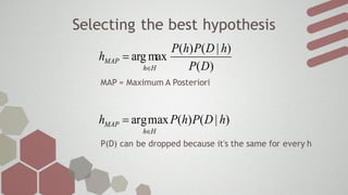
Bayesian learning allows systems to classify new examples based on a model learned from prior examples using probabilities. It reasons by calculating the posterior probability of a hypothesis given new evidence using Bayes' rule. The maximum a posteriori (MAP) hypothesis that best explains the evidence is selected. Naive Bayes classifiers make a strong independence assumption between attributes. They classify new examples by calculating the posterior probability of each class and choosing the class with the highest value. Overfitting can occur if the learned model is too complex for the data. Model selection aims to avoid overfitting by evaluating models on separate training and test datasets.

1. Bayesian Learning

2. A sample learning task: Classification
• The system is given a set of instances to learn from
• The system builds/selects a model/hypothesis based
on the given instances
• Based on the learned model the system can classify
unseen instances

3. Reasoning with probabilities
)(
)|()(
)|(
DP
hDPhP
DhP 
Bayes Rule
evidence
likelihoodprior
posterior



4. Selecting the best hypothesis
)|()(maxarg hDPhPh
Hh
MAP


)(
)|()(
maxarg
DP
hDPhP
h
Hh
MAP


P(D) can be dropped because it's the same for every h
MAP = Maximum A Posteriori

5. Probability of Poliposis
008.0)( poliposisP
98.0)|(  poliposisP
0078.0008.098.0)|()(  poliposisPpoliposisP
?)|( poliposisP
Given a medical test is positive what's the probability
we actually have polisposis disease?
prior
likelihood
posterior

6. Probability of Poliposis
992.0)( poliposisP
03.0)|(  poliposisP
0298.0992.003.0)|()(  poliposisPpoliposisP
?)|( poliposisP
prior
likelihood
posterior
Given a medical test is positive what's the probability
we DON'T have polisposis disease?

7. Probability of Poliposis
0078.0)|()(  poliposisPpoliposisP
0298.0)|()(  poliposisPpoliposisP
21.0)|( poliposisP
By normalizing we obtain the above probabilities.
It's approximately 4 times more likely we DON'T have polisposis
By comparing the posteriors we find the map hypothesis
79.0)|( poliposisP

8. Learning from examples
Day Outlook Temp Humidity Wind Play Hacky Sack
1 Sunny Hot High Weak Yes
2 Sunny Hot High Strong No
3 Overcast Hot High Strong Yes
4 Rain Mild High Strong no
5 Rain Cool Normal Strong No
6 Rain Cool Normal Strong No

9. Naive Bayes classifier
)|()(maxarg hDPhPh
Hh
MAP




i
kik
Kk
NB CxPCPC )|()(maxarg
Called naive because it assumes all attributes are independent

10. Implicit model
Day Outlook Temp Humidity Wind Class
1 Sunny = 1/2
Hot = 2/2 High = 2/2
Weak = 1/2
Yes= 2/6
3 Overcast= 1/2 Strong = 1/2
2 Sunny = 1/4 Hot = 1/4
High = 2/4
Strong = 4/4 No = 4/6
4
Rain = 3/4
Mild = 1/4
5
Cool = 2/4 Normal = 2/4
6

11. Classifying an example
333.06/2)(  yesackPlayHackySP
Day Outlook Temp Humidity Wind Play Hacky Sack?
7 Sunny Hot High Strong ?
666.06/4)(  noackPlayHackySP
5.02/1)|(  yesackPlayHackySsunnyOutlookP
25.04/1)|(  noackPlayHackySsunnyOutlookP
12/2)|(  yesackPlayHackyShotTempP
25.04/1)|(  noackPlayHackyShotTempP
12/2)|(  yesackPlayHackyShighHumidityP
5.04/2)|(  noackPlayHackyShighHumidityP
5.02/1)|(  yesackPlayHackySstrongWindP
14/4)|(  noackPlayHackySstrongWindP
prior
likelihood

12. Result
08325.05.0115.0333.0)|()|()|()|()( yesstrongPyeshighPyeshotPyessunnyPyesP
8.0! yesackPlayHackyS
0208125.015.025.025.0666.0)|()|()|()|()( nostrongPnohighPnohotPnosunnyPnoP
Calculating the MAP hypothesis for class 'yes' & 'no'

13. Least square error hypothesis
Where the red lines represents the error

14. Choosing between two hypotheses
red/yellow lines are the error for h1/h2

15. Maximum Likelihood Hypothesis
)|(maxarg hDPh
Hh
ML




m
i
i
Hh
ML hdPh
1
)|(maxarg
Assuming all data points are independent
Assuming uniform priors

16. Least square error hypothesis
2
2
))((
2
1
1
2
2
1
maxarg
ii xhdm
iHh
ML eh


 

using a least square error method has a profound theoretical basis


m
i
ii
Hh
ML xhdh
1
2
))((minarg
assuming the noise is normally distributed

17. Squared error analysis
x error h1 error h2 square e1 square e2
2 -1.5 2 2.25 4
4 4.5 6 20.25 36
6 -1.5 -2 2.25 4
8 1.5 -1 2.25 1
10 6.5 2 42.25 4
product 9745.39 2304
h2 is more likely then h1 since it has a smaller
squared error product

18. Overfitting
The model found by the learning algorithm is too complex

19. Model selection
• Usually tested by splitting the data into training and
testing examples
• Do model selection based on different data sets
• Prefer simple hypothesis over more complex ones
(assign lower priors to complex hypothesis)

20. Minimum Description Length learning
(MDL)
• Encode both hypothesis and data using an optimal
encoding will output the MAP hypothesis.
)|()(minarg 21
hDLhLh CC
Hh
MDL 

MAPMDL hh 
Compression, Probability, Regularity are all closely related!

21. References
• Tom M. Mitchell (1997) Machine Learning (pp 154-200)