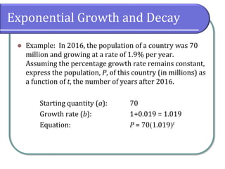
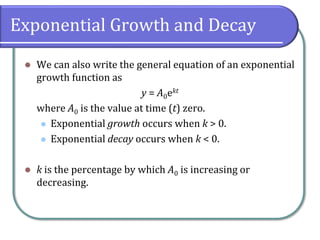
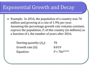
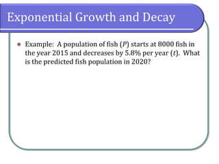
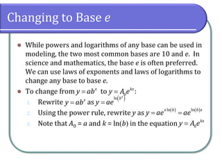
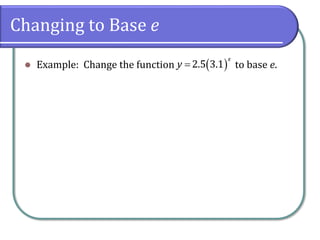
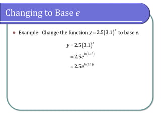
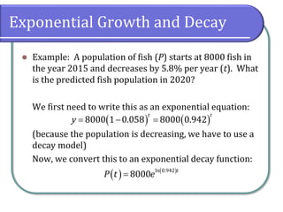
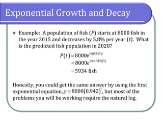
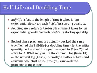
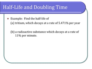
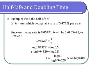
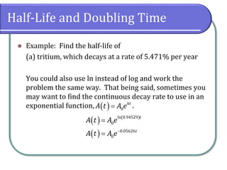
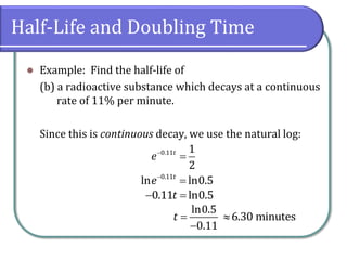
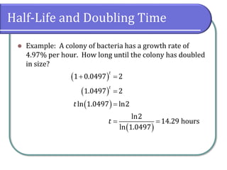
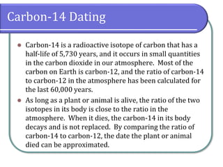
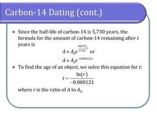
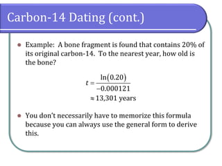
* Model exponential growth and decay.
* Use Newton’s Law of Cooling.
* Use logistic-growth models.
* Choose an appropriate model for data.
* Express an exponential model in base e.
* Model exponential growth and decay.
* Use Newton’s Law of Cooling.
* Use logistic-growth models.
* Choose an appropriate model for data.
* Express an exponential model in base e.
This document discusses exponential growth and decay functions. It provides examples of how to set up and solve exponential equations to model population growth, fish population decline, and bacterial growth. It also explains how to calculate half-life, which is the time for an exponentially decaying quantity to reduce to half its initial value, and doubling time. Examples are worked through to find the half-life of tritium and a radioactive substance, and to determine the amount of a radioactive substance remaining after a given number of years based on its known half-life. The document concludes with classwork practice problems listed from the textbook.
This document discusses exponential growth and decay functions. It provides examples of how to set up and solve exponential equations to model population growth, fish population decline, world poultry production increase, and bacterial growth. It also explains how to calculate half-life and doubling time for exponential decay and growth. Examples are worked through to find the half-life of tritium decaying at 5.471% per year and a radioactive substance decaying at 11% per minute, and to determine the amount of radioactive substance remaining after 6 years given its half-life is 3 years. The document concludes with assignments for students.
This document discusses first-order differential equations. It provides exercises related to modeling real-world phenomena using differential equations, including population growth, radioactive decay, learning rates, and exponential growth. It also covers equilibrium solutions and determining whether a solution is increasing or decreasing based on the sign of the derivative. Key concepts covered are modeling, equilibrium solutions, exponential functions, and interpreting solutions.
The document discusses exponential functions and their applications to modeling real-world situations involving population growth, radioactive decay, and compound interest. Exponential functions have the variable in the exponent and have properties like being one-to-one that allow equations with them to be solved. Examples are worked through to demonstrate how to set up and solve exponential models for situations involving doubling populations, radioactive half-life, and compound interest calculations.
The document discusses exponential and natural logarithm functions. It provides examples of using exponential functions to calculate continuous compound interest on investments over time, and shows that continuous compounding yields slightly higher returns. It also discusses properties of the natural logarithm function and its relationship to the exponential function. An example calculates the area under a curve bounded by lines using the natural logarithm formula.
August 7, 2012 2103 c02 Sheet number 30 Page number 60 cyan b.docxrock73
August 7, 2012 21:03 c02 Sheet number 30 Page number 60 cyan black
60 Chapter 2. First Order Differential Equations
Solving Eq. (31) for v0, we find the initial velocity required to lift the body to the altitude ξ,
namely,
v0 =
√
2gR
ξ
R + ξ . (32)
The escape velocity ve is then found by letting ξ → ∞. Consequently,
ve =
√
2gR. (33)
The numerical value of ve is approximately 6.9 mi/s, or 11.1 km/s.
The preceding calculation of the escape velocity neglects the effect of air resistance, so the
actual escape velocity (including the effect of air resistance) is somewhat higher. On the other
hand, the effective escape velocity can be significantly reduced if the body is transported a
considerable distance above sea level before being launched. Both gravitational and frictional
forces are thereby reduced;air resistance, in particular,diminishes quite rapidly with increasing
altitude. You should keep in mind also that it may well be impractical to impart too large an
initial velocity instantaneously; space vehicles, for instance, receive their initial acceleration
during a period of a few minutes.
PROBLEMS 1. Consider a tank used in certain hydrodynamic experiments. After one experiment the
tank contains 200 L of a dye solution with a concentration of 1 g/L. To prepare for
the next experiment, the tank is to be rinsed with fresh water flowing in at a rate of
2 L/min, the well-stirred solution flowing out at the same rate. Find the time that will
elapse before the concentration of dye in the tank reaches 1% of its original value.
2. A tank initially contains 120 L of pure water. A mixture containing a concentration of
γ g/L of salt enters the tank at a rate of 2 L/min, and the well-stirred mixture leaves the
tank at the same rate. Find an expression in terms of γ for the amount of salt in the tank
at any time t. Also find the limiting amount of salt in the tank as t → ∞.
3. A tank originally contains 100 gal of fresh water. Then water containing 12 lb of salt per
gallon is poured into the tank at a rate of 2 gal/min, and the mixture is allowed to leave at
the same rate. After 10 min the process is stopped, and fresh water is poured into the tank
at a rate of 2 gal/min, with the mixture again leaving at the same rate. Find the amount of
salt in the tank at the end of an additional 10 min.
4. A tank with a capacity of 500 gal originally contains 200 gal of water with 100 lb of salt
in solution. Water containing 1 lb of salt per gallon is entering at a rate of 3 gal/min, and
the mixture is allowed to flow out of the tank at a rate of 2 gal/min. Find the amount
of salt in the tank at any time prior to the instant when the solution begins to overflow.
Find the concentration (in pounds per gallon) of salt in the tank when it is on the point
of overflowing. Compare this concentration with the theoretical limiting concentration if
the tank had infinite capacity.
5. A tank contains 100 gal of water and 50 oz of salt. Water containing a salt con ...
The document discusses exponential growth and decay models. Exponential growth models use the formula y = C(1 + r)t, where C is the initial amount, t is time, r is the growth rate, and (1 + r) is the growth factor. Exponential decay models use the formula y = C(1 - r)t, where (1 - r) is the decay factor and r is the decay rate. Examples are provided to demonstrate how to write, graph, and apply these models to problems involving compound interest, population growth, radioactive decay, and purchasing power.
The document discusses exponential and logarithmic functions. It defines logarithms as exponents and explains that logarithms were once used to simplify calculations before calculators. It then covers several topics related to exponential functions including:
- Basic laws of exponents using integral exponents
- Examples of applying the order of operations to exponents
- Extending the rules of exponents to include rational exponents
- Exponential growth and decay models and examples
- Graphing and properties of exponential functions
- The number e and the natural exponential function ex
- Compound interest formulas including continuous compounding
Lesson 15: Exponential Growth and Decay (slides)Matthew Leingang
Many problems in nature are expressible in terms of a certain differential equation that has a solution in terms of exponential functions. We look at the equation in general and some fun applications, including radioactivity, cooling, and interest.
* Evaluate exponential functions.
* Find the equation of an exponential function.
* Use compound interest formulas.
* Evaluate exponential functions with base e.
The document reviews exponential functions and their applications. It defines an exponential function as a function of the form f(x) = bx, where b > 0 and b ≠ 1. Exponential functions can model real-life situations involving population growth, radioactive decay, and compound interest over time. Examples are provided to demonstrate how to write exponential functions and solve equations to model various applications involving exponential growth or decay.
The document discusses exponential functions, equations, and inequalities. It provides examples of common applications of exponential functions in real life like population growth, exponential decay, and compound interest. It also gives examples of exponential models for population growth, exponential decay of radioactive substances, and compound interest. The last part defines the natural exponential function and provides an example of predicting population using an exponential function.
This document discusses applications of first and second order differential equations. It covers several topics:
1. Newton's Law of Cooling - Describes how the rate of change of an object's temperature is proportional to the difference between its temperature and the ambient temperature.
2. Radioactive Decay - The rate of decay of a radioactive material is proportional to the amount present.
3. RC and LR Circuits - Differential equations model the charging and discharging behavior of capacitors and inductors in circuits.
4. Forced Oscillations and Resonance - Differential equations are used to model forced vibrations and resonance phenomena in oscillating systems like LCR circuits.
This document provides the solution to an exponential modeling problem using the compound interest formula. It shows that if $10,000 is invested at a 10% annual interest rate and compounds annually, it would take approximately 48 years to grow to $1,000,000. The key steps are:
1) Setting up the compound interest formula with the known values of principal, interest rate, and future value.
2) Taking the log of both sides to isolate the unknown time variable since it is an exponent.
3) Calculating the value of t as approximately 48 years.
The document discusses exponential functions and how they can be used to model real-world situations involving growth and decay over time. Exponential functions take the form of y = abx or f(x) = abx, where b is the base. Common bases used are 2 to model doubling and e to model continuous growth/decay. Examples are given of exponential functions modeling population growth, radioactive decay, and compound interest. Exponential equations and inequalities can be solved for x, while exponential functions express a relationship between variables.
Applications of Differential Equations of First order and First DegreeDheirya Joshi
The document describes how to calculate the time it takes for a population growing at 5% annually to double in size using a differential equation model. It is also solved to be 20loge2 years, or approximately 14 years. A second problem involves calculating the final temperature of liquid in an insulated cylindrical tank over 5 days using a heat transfer model. A third problem uses kinematics equations to find how far a drag racer will travel in 8 seconds if its speed increases by 40 feet per second each second.
Intro to physical science and measurementssihellyay
This document provides an introduction to physical science. It begins by defining science and listing the main branches - biological science, physical science, and social science. Biological science deals with living things, social science deals with human behavior and societies. Physical science deals with non-living things, their composition, nature, characteristics, and changes.
The main branches of physical science are then defined: chemistry studies matter and its properties/structure/changes, physics studies matter and energy/their interactions, astronomy studies the universe/heavenly bodies, geology studies Earth materials/structures/processes, and meteorology studies the atmosphere/weather/climate.
The document then moves to a chapter about measurement, defining it as collecting quantitative data by
This document provides an introduction to physical science. It begins by defining science and listing the main branches - biological science, physical science, and social science. Biological science deals with living things, social science deals with human behavior and societies. Physical science deals with non-living things, their properties, structures, and changes.
The main branches of physical science are then outlined as chemistry, physics, astronomy, geology, and meteorology. Chemistry studies matter and its properties and changes. Physics studies matter and energy. Astronomy studies the universe and celestial bodies. Geology studies Earth materials, structures, and processes. Meteorology studies the atmosphere and weather/climate.
The document then transitions to discussing measurement in physical science. Measurement
- A ratio compares two quantities with the same unit and can be written as a fraction, with a colon, or using "to".
- A rate compares two quantities with different units and is written as a fraction with units.
- A proportion states that two ratios or rates are equal, and can be solved by setting the cross products equal.
- Unit rates have the denominator simplified to 1 and often use "per" to express the comparison.
The document discusses several engineering problems involving mathematical modeling and problem solving techniques. It provides examples of using concepts like material balances, decay rates, Newton's law of cooling, Euler's method, Taylor series approximations, and finite difference methods to model and solve problems related to water balance in the human body, falling parachutists, radioactive decay, heat transfer, evaporation, fluid flow in storage tanks, numerical approximations, and missile trajectories.
The document discusses several engineering problems involving mathematical modeling and problem solving techniques. It provides examples of using concepts like material balances, decay rates, Newton's law of cooling, Euler's method, Taylor series approximations, and finite difference methods to model and solve problems related to water balance in the human body, falling parachutists, radioactive decay, heat transfer, evaporation, fluid flow, numerical approximations, and missile trajectories.
This document discusses exponential functions and their applications to modeling compound interest, population growth, radioactive decay, and dating artifacts. It provides definitions of compound interest, continuous compounding, and exponential decay models. Examples are given to illustrate using these models to calculate amounts with compound interest over time, population sizes over generations, radioactive material half-life decay, and estimating the ages of artifacts based on their remaining radioactive carbon.
The document discusses population growth and decay models including Malthusian, radioactive decay, and logistic growth models. It provides examples of calculating growth/decay rates, population sizes over time, and half-lives using the various formulas. Key models covered include Malthusian growth, radioactive decay based on half-life, and carbon-14 dating to estimate the age of living things.
This document provides an overview of key concepts from the first chapter of a physics textbook. It introduces why physics is studied, important terminology in physics, use of mathematics in physics, scientific notation and significant figures, units and dimensional analysis, problem-solving techniques, and graphing. Examples are provided for many topics to illustrate physics concepts and calculations involving units, proportions, percentages, and graphing patient temperature data.
* Model exponential growth and decay
* Use Newton's Law of Cooling
* Use logistic-growth models
* Choose an appropriate model for data
* Express an exponential model in base e
* Construct perpendicular and angle bisectors
* Use bisectors to solve problems
* Identify the circumcenter and incenter of a triangle
* Use triangle segments to solve problems
The document discusses exponential growth and decay models. Exponential growth models use the formula y = C(1 + r)t, where C is the initial amount, t is time, r is the growth rate, and (1 + r) is the growth factor. Exponential decay models use the formula y = C(1 - r)t, where (1 - r) is the decay factor and r is the decay rate. Examples are provided to demonstrate how to write, graph, and apply these models to problems involving compound interest, population growth, radioactive decay, and purchasing power.
The document discusses exponential and logarithmic functions. It defines logarithms as exponents and explains that logarithms were once used to simplify calculations before calculators. It then covers several topics related to exponential functions including:
- Basic laws of exponents using integral exponents
- Examples of applying the order of operations to exponents
- Extending the rules of exponents to include rational exponents
- Exponential growth and decay models and examples
- Graphing and properties of exponential functions
- The number e and the natural exponential function ex
- Compound interest formulas including continuous compounding
Lesson 15: Exponential Growth and Decay (slides)Matthew Leingang
Many problems in nature are expressible in terms of a certain differential equation that has a solution in terms of exponential functions. We look at the equation in general and some fun applications, including radioactivity, cooling, and interest.
* Evaluate exponential functions.
* Find the equation of an exponential function.
* Use compound interest formulas.
* Evaluate exponential functions with base e.
The document reviews exponential functions and their applications. It defines an exponential function as a function of the form f(x) = bx, where b > 0 and b ≠ 1. Exponential functions can model real-life situations involving population growth, radioactive decay, and compound interest over time. Examples are provided to demonstrate how to write exponential functions and solve equations to model various applications involving exponential growth or decay.
The document discusses exponential functions, equations, and inequalities. It provides examples of common applications of exponential functions in real life like population growth, exponential decay, and compound interest. It also gives examples of exponential models for population growth, exponential decay of radioactive substances, and compound interest. The last part defines the natural exponential function and provides an example of predicting population using an exponential function.
This document discusses applications of first and second order differential equations. It covers several topics:
1. Newton's Law of Cooling - Describes how the rate of change of an object's temperature is proportional to the difference between its temperature and the ambient temperature.
2. Radioactive Decay - The rate of decay of a radioactive material is proportional to the amount present.
3. RC and LR Circuits - Differential equations model the charging and discharging behavior of capacitors and inductors in circuits.
4. Forced Oscillations and Resonance - Differential equations are used to model forced vibrations and resonance phenomena in oscillating systems like LCR circuits.
This document provides the solution to an exponential modeling problem using the compound interest formula. It shows that if $10,000 is invested at a 10% annual interest rate and compounds annually, it would take approximately 48 years to grow to $1,000,000. The key steps are:
1) Setting up the compound interest formula with the known values of principal, interest rate, and future value.
2) Taking the log of both sides to isolate the unknown time variable since it is an exponent.
3) Calculating the value of t as approximately 48 years.
The document discusses exponential functions and how they can be used to model real-world situations involving growth and decay over time. Exponential functions take the form of y = abx or f(x) = abx, where b is the base. Common bases used are 2 to model doubling and e to model continuous growth/decay. Examples are given of exponential functions modeling population growth, radioactive decay, and compound interest. Exponential equations and inequalities can be solved for x, while exponential functions express a relationship between variables.
Applications of Differential Equations of First order and First DegreeDheirya Joshi
The document describes how to calculate the time it takes for a population growing at 5% annually to double in size using a differential equation model. It is also solved to be 20loge2 years, or approximately 14 years. A second problem involves calculating the final temperature of liquid in an insulated cylindrical tank over 5 days using a heat transfer model. A third problem uses kinematics equations to find how far a drag racer will travel in 8 seconds if its speed increases by 40 feet per second each second.
Intro to physical science and measurementssihellyay
This document provides an introduction to physical science. It begins by defining science and listing the main branches - biological science, physical science, and social science. Biological science deals with living things, social science deals with human behavior and societies. Physical science deals with non-living things, their composition, nature, characteristics, and changes.
The main branches of physical science are then defined: chemistry studies matter and its properties/structure/changes, physics studies matter and energy/their interactions, astronomy studies the universe/heavenly bodies, geology studies Earth materials/structures/processes, and meteorology studies the atmosphere/weather/climate.
The document then moves to a chapter about measurement, defining it as collecting quantitative data by
This document provides an introduction to physical science. It begins by defining science and listing the main branches - biological science, physical science, and social science. Biological science deals with living things, social science deals with human behavior and societies. Physical science deals with non-living things, their properties, structures, and changes.
The main branches of physical science are then outlined as chemistry, physics, astronomy, geology, and meteorology. Chemistry studies matter and its properties and changes. Physics studies matter and energy. Astronomy studies the universe and celestial bodies. Geology studies Earth materials, structures, and processes. Meteorology studies the atmosphere and weather/climate.
The document then transitions to discussing measurement in physical science. Measurement
- A ratio compares two quantities with the same unit and can be written as a fraction, with a colon, or using "to".
- A rate compares two quantities with different units and is written as a fraction with units.
- A proportion states that two ratios or rates are equal, and can be solved by setting the cross products equal.
- Unit rates have the denominator simplified to 1 and often use "per" to express the comparison.
The document discusses several engineering problems involving mathematical modeling and problem solving techniques. It provides examples of using concepts like material balances, decay rates, Newton's law of cooling, Euler's method, Taylor series approximations, and finite difference methods to model and solve problems related to water balance in the human body, falling parachutists, radioactive decay, heat transfer, evaporation, fluid flow in storage tanks, numerical approximations, and missile trajectories.
The document discusses several engineering problems involving mathematical modeling and problem solving techniques. It provides examples of using concepts like material balances, decay rates, Newton's law of cooling, Euler's method, Taylor series approximations, and finite difference methods to model and solve problems related to water balance in the human body, falling parachutists, radioactive decay, heat transfer, evaporation, fluid flow, numerical approximations, and missile trajectories.
This document discusses exponential functions and their applications to modeling compound interest, population growth, radioactive decay, and dating artifacts. It provides definitions of compound interest, continuous compounding, and exponential decay models. Examples are given to illustrate using these models to calculate amounts with compound interest over time, population sizes over generations, radioactive material half-life decay, and estimating the ages of artifacts based on their remaining radioactive carbon.
The document discusses population growth and decay models including Malthusian, radioactive decay, and logistic growth models. It provides examples of calculating growth/decay rates, population sizes over time, and half-lives using the various formulas. Key models covered include Malthusian growth, radioactive decay based on half-life, and carbon-14 dating to estimate the age of living things.
This document provides an overview of key concepts from the first chapter of a physics textbook. It introduces why physics is studied, important terminology in physics, use of mathematics in physics, scientific notation and significant figures, units and dimensional analysis, problem-solving techniques, and graphing. Examples are provided for many topics to illustrate physics concepts and calculations involving units, proportions, percentages, and graphing patient temperature data.
Similar to 6.7 Exponential and Logarithmic Models (20)
* Model exponential growth and decay
* Use Newton's Law of Cooling
* Use logistic-growth models
* Choose an appropriate model for data
* Express an exponential model in base e
* Construct perpendicular and angle bisectors
* Use bisectors to solve problems
* Identify the circumcenter and incenter of a triangle
* Use triangle segments to solve problems
* Identify, write, and analyze conditional statements
* Write the inverse, converse, and contrapositive of a conditional statement
* Write a counterexample to a fake conjecture
* Find the distance between two points
* Find the midpoint of two given points
* Find the coordinates of an endpoint given one endpoint and a midpoint
* Find the coordinates of a point a fractional distance from one end of a segment
This document provides instruction on factoring polynomials and quadratic equations. It begins by reviewing factoring techniques like finding the greatest common factor and factoring trinomials and binomials. Examples are provided to demonstrate the factoring methods. The document then discusses solving quadratic equations by factoring, putting the equation in standard form, and setting each factor equal to zero. An example problem demonstrates solving a quadratic equation through factoring. The document concludes by assigning homework and an optional reading for the next class.
* Connect functions to their graphs
* Graph piecewise-defined functions
* Graph absolute value functions
* Graph greatest-integer functions
* Interpret graphs
* Use the vertical line test to determine a function
* Connect functions to their graphs
* Graph piecewise-defined functions
* Graph absolute value functions
* Graph greatest-integer functions
* Interpret graphs
* Use the vertical line test to determine a function
* Introduce functions and function notation
* Develop skills in constructing and interpreting the graphs of functions
* Learn to apply this knowledge in a variety of situations
* Recognize graphs of common functions.
* Graph functions using vertical and horizontal shifts.
* Graph functions using reflections about the x-axis and the y-axis.
* Graph functions using compressions and stretches.
* Combine transformations.
This document discusses functions and their graphs. It defines increasing, decreasing and constant functions based on how the function values change as the input increases. Relative maxima and minima are points where a function changes from increasing to decreasing. Symmetry of functions is classified by the y-axis, x-axis and origin. Even functions are symmetric about the y-axis, odd functions are symmetric about the origin. Piecewise functions have different definitions over different intervals.
This document provides examples and steps for solving various types of equations beyond linear equations, including:
1) Polynomial equations solved by factoring
2) Equations with radicals where radicals are eliminated by raising both sides to a power
3) Equations with rational exponents where both sides are raised to the reciprocal power
4) Equations quadratic in form where an algebraic substitution is made to transform into a quadratic equation
5) Absolute value equations where both positive and negative solutions must be considered.
This document provides instruction on factoring quadratic equations. It begins by reviewing factoring polynomials and trinomials. It then discusses factoring binomials using difference of squares, sum/difference of cubes, and other patterns. Finally, it explains that a quadratic equation can be solved by factoring if it can be written as a product of two linear factors. An example demonstrates factoring a quadratic equation by finding the two values that make each factor equal to zero.
This document provides an overview of functions and their graphs. It defines what constitutes a function, discusses domain and range, and how to identify functions using the vertical line test. Key points covered include:
- A function is a relation where each input has a single, unique output
- The domain is the set of inputs and the range is the set of outputs
- Functions can be represented by ordered pairs, graphs, or equations
- The vertical line test identifies functions as those where a vertical line intersects the graph at most once
- Intercepts occur where the graph crosses the x or y-axis
The document discusses the binomial theorem, which provides a formula for expanding binomial expressions of the form (a + b)^n. It gives the formula for finding the coefficient of the term containing b^r as nCr. Several examples are worked out applying the binomial theorem to expand binomial expressions and find specific terms. Factorial notation is introduced for writing the coefficients. The document also discusses using calculators and Desmos to evaluate binomial coefficients. Practice problems are assigned from previous sections.
The document discusses using Venn diagrams and two-way tables to organize data and calculate probabilities. It provides examples of completing Venn diagrams and two-way tables based on survey data about students' activities. It then uses the tables and diagrams to calculate probabilities of different outcomes. The examples illustrate how to set up and use these visual representations of categorical data.
* Solve counting problems using the Addition Principle.
* Solve counting problems using the Multiplication Principle.
* Solve counting problems using permutations involving n distinct objects.
* Solve counting problems using combinations.
* Find the number of subsets of a given set.
* Solve counting problems using permutations involving n non-distinct objects.
* Use summation notation.
* Use the formula for the sum of the first n terms of an arithmetic series.
* Use the formula for the sum of the first n terms of a geometric series.
* Use the formula for the sum of an infinite geometric series.
* Solve annuity problems.
* Find the common ratio for a geometric sequence.
* List the terms of a geometric sequence.
* Use a recursive formula for a geometric sequence.
* Use an explicit formula for a geometric sequence.
How to Setup Warehouse & Location in Odoo 17 InventoryCeline George
In this slide, we'll explore how to set up warehouses and locations in Odoo 17 Inventory. This will help us manage our stock effectively, track inventory levels, and streamline warehouse operations.
How to Manage Your Lost Opportunities in Odoo 17 CRMCeline George
Odoo 17 CRM allows us to track why we lose sales opportunities with "Lost Reasons." This helps analyze our sales process and identify areas for improvement. Here's how to configure lost reasons in Odoo 17 CRM
Chapter wise All Notes of First year Basic Civil Engineering.pptxDenish Jangid
Chapter wise All Notes of First year Basic Civil Engineering
Syllabus
Chapter-1
Introduction to objective, scope and outcome the subject
Chapter 2
Introduction: Scope and Specialization of Civil Engineering, Role of civil Engineer in Society, Impact of infrastructural development on economy of country.
Chapter 3
Surveying: Object Principles & Types of Surveying; Site Plans, Plans & Maps; Scales & Unit of different Measurements.
Linear Measurements: Instruments used. Linear Measurement by Tape, Ranging out Survey Lines and overcoming Obstructions; Measurements on sloping ground; Tape corrections, conventional symbols. Angular Measurements: Instruments used; Introduction to Compass Surveying, Bearings and Longitude & Latitude of a Line, Introduction to total station.
Levelling: Instrument used Object of levelling, Methods of levelling in brief, and Contour maps.
Chapter 4
Buildings: Selection of site for Buildings, Layout of Building Plan, Types of buildings, Plinth area, carpet area, floor space index, Introduction to building byelaws, concept of sun light & ventilation. Components of Buildings & their functions, Basic concept of R.C.C., Introduction to types of foundation
Chapter 5
Transportation: Introduction to Transportation Engineering; Traffic and Road Safety: Types and Characteristics of Various Modes of Transportation; Various Road Traffic Signs, Causes of Accidents and Road Safety Measures.
Chapter 6
Environmental Engineering: Environmental Pollution, Environmental Acts and Regulations, Functional Concepts of Ecology, Basics of Species, Biodiversity, Ecosystem, Hydrological Cycle; Chemical Cycles: Carbon, Nitrogen & Phosphorus; Energy Flow in Ecosystems.
Water Pollution: Water Quality standards, Introduction to Treatment & Disposal of Waste Water. Reuse and Saving of Water, Rain Water Harvesting. Solid Waste Management: Classification of Solid Waste, Collection, Transportation and Disposal of Solid. Recycling of Solid Waste: Energy Recovery, Sanitary Landfill, On-Site Sanitation. Air & Noise Pollution: Primary and Secondary air pollutants, Harmful effects of Air Pollution, Control of Air Pollution. . Noise Pollution Harmful Effects of noise pollution, control of noise pollution, Global warming & Climate Change, Ozone depletion, Greenhouse effect
Text Books:
1. Palancharmy, Basic Civil Engineering, McGraw Hill publishers.
2. Satheesh Gopi, Basic Civil Engineering, Pearson Publishers.
3. Ketki Rangwala Dalal, Essentials of Civil Engineering, Charotar Publishing House.
4. BCP, Surveying volume 1
LAND USE LAND COVER AND NDVI OF MIRZAPUR DISTRICT, UPRAHUL
This Dissertation explores the particular circumstances of Mirzapur, a region located in the
core of India. Mirzapur, with its varied terrains and abundant biodiversity, offers an optimal
environment for investigating the changes in vegetation cover dynamics. Our study utilizes
advanced technologies such as GIS (Geographic Information Systems) and Remote sensing to
analyze the transformations that have taken place over the course of a decade.
The complex relationship between human activities and the environment has been the focus
of extensive research and worry. As the global community grapples with swift urbanization,
population expansion, and economic progress, the effects on natural ecosystems are becoming
more evident. A crucial element of this impact is the alteration of vegetation cover, which plays a
significant role in maintaining the ecological equilibrium of our planet.Land serves as the foundation for all human activities and provides the necessary materials for
these activities. As the most crucial natural resource, its utilization by humans results in different
'Land uses,' which are determined by both human activities and the physical characteristics of the
land.
The utilization of land is impacted by human needs and environmental factors. In countries
like India, rapid population growth and the emphasis on extensive resource exploitation can lead
to significant land degradation, adversely affecting the region's land cover.
Therefore, human intervention has significantly influenced land use patterns over many
centuries, evolving its structure over time and space. In the present era, these changes have
accelerated due to factors such as agriculture and urbanization. Information regarding land use and
cover is essential for various planning and management tasks related to the Earth's surface,
providing crucial environmental data for scientific, resource management, policy purposes, and
diverse human activities.
Accurate understanding of land use and cover is imperative for the development planning
of any area. Consequently, a wide range of professionals, including earth system scientists, land
and water managers, and urban planners, are interested in obtaining data on land use and cover
changes, conversion trends, and other related patterns. The spatial dimensions of land use and
cover support policymakers and scientists in making well-informed decisions, as alterations in
these patterns indicate shifts in economic and social conditions. Monitoring such changes with the
help of Advanced technologies like Remote Sensing and Geographic Information Systems is
crucial for coordinated efforts across different administrative levels. Advanced technologies like
Remote Sensing and Geographic Information Systems
9
Changes in vegetation cover refer to variations in the distribution, composition, and overall
structure of plant communities across different temporal and spatial scales. These changes can
occur natural.
This slide is special for master students (MIBS & MIFB) in UUM. Also useful for readers who are interested in the topic of contemporary Islamic banking.
বাংলাদেশের অর্থনৈতিক সমীক্ষা ২০২৪ [Bangladesh Economic Review 2024 Bangla.pdf] কম্পিউটার , ট্যাব ও স্মার্ট ফোন ভার্সন সহ সম্পূর্ণ বাংলা ই-বুক বা pdf বই " সুচিপত্র ...বুকমার্ক মেনু 🔖 ও হাইপার লিংক মেনু 📝👆 যুক্ত ..
আমাদের সবার জন্য খুব খুব গুরুত্বপূর্ণ একটি বই ..বিসিএস, ব্যাংক, ইউনিভার্সিটি ভর্তি ও যে কোন প্রতিযোগিতা মূলক পরীক্ষার জন্য এর খুব ইম্পরট্যান্ট একটি বিষয় ...তাছাড়া বাংলাদেশের সাম্প্রতিক যে কোন ডাটা বা তথ্য এই বইতে পাবেন ...
তাই একজন নাগরিক হিসাবে এই তথ্য গুলো আপনার জানা প্রয়োজন ...।
বিসিএস ও ব্যাংক এর লিখিত পরীক্ষা ...+এছাড়া মাধ্যমিক ও উচ্চমাধ্যমিকের স্টুডেন্টদের জন্য অনেক কাজে আসবে ...
Beyond Degrees - Empowering the Workforce in the Context of Skills-First.pptxEduSkills OECD
Iván Bornacelly, Policy Analyst at the OECD Centre for Skills, OECD, presents at the webinar 'Tackling job market gaps with a skills-first approach' on 12 June 2024
Walmart Business+ and Spark Good for Nonprofits.pdfTechSoup
"Learn about all the ways Walmart supports nonprofit organizations.
You will hear from Liz Willett, the Head of Nonprofits, and hear about what Walmart is doing to help nonprofits, including Walmart Business and Spark Good. Walmart Business+ is a new offer for nonprofits that offers discounts and also streamlines nonprofits order and expense tracking, saving time and money.
The webinar may also give some examples on how nonprofits can best leverage Walmart Business+.
The event will cover the following::
Walmart Business + (https://business.walmart.com/plus) is a new shopping experience for nonprofits, schools, and local business customers that connects an exclusive online shopping experience to stores. Benefits include free delivery and shipping, a 'Spend Analytics” feature, special discounts, deals and tax-exempt shopping.
Special TechSoup offer for a free 180 days membership, and up to $150 in discounts on eligible orders.
Spark Good (walmart.com/sparkgood) is a charitable platform that enables nonprofits to receive donations directly from customers and associates.
Answers about how you can do more with Walmart!"
2. Concepts and Objectives
⚫ Objectives for this section are
⚫ Model exponential growth and decay.
⚫ Use Newton’s Law of Cooling.
⚫ Use logistic-growth models.
⚫ Choose an appropriate model for data.
⚫ Express an exponential model in base e.
3. Exponential Growth and Decay
⚫ The general equation of an exponential function is
y = abx
where a and b are constants.
⚫ Exponential growth occurs when b > 1.
⚫ Exponential decay occurs when 0 < b < 1.
⚫ The constant a is usually the starting value and b is the
percentage by which a is increasing or decreasing.
4. Exponential Growth and Decay
⚫ Example: In 2016, the population of a country was 70
million and growing at a rate of 1.9% per year.
Assuming the percentage growth rate remains constant,
express the population, P, of this country (in millions) as
a function of t, the number of years after 2016.
5. Exponential Growth and Decay
⚫ Example: In 2016, the population of a country was 70
million and growing at a rate of 1.9% per year.
Assuming the percentage growth rate remains constant,
express the population, P, of this country (in millions) as
a function of t, the number of years after 2016.
Starting quantity (a): 70
Growth rate (b): 1+0.019 = 1.019
Equation: P = 70(1.019)t
6. Exponential Growth and Decay
⚫ We can also write the general equation of an exponential
growth function as
y = A0ekt
where A0 is the value at time (t) zero.
⚫ Exponential growth occurs when k > 0.
⚫ Exponential decay occurs when k < 0.
⚫ k is the percentage by which A0 is increasing or
decreasing.
7. Exponential Growth and Decay
⚫ Example: In 2016, the population of a country was 70
million and growing at a rate of 1.9% per year.
Assuming the percentage growth rate remains constant,
express the population, P, of this country (in millions) as
a function of t, the number of years after 2016.
8. Exponential Growth and Decay
⚫ Example: In 2016, the population of a country was 70
million and growing at a rate of 1.9% per year.
Assuming the percentage growth rate remains constant,
express the population, P, of this country (in millions) as
a function of t, the number of years after 2016.
Starting quantity (A0): 70
Growth rate (k): 0.019
Equation: P = 70e0.019t
9. Exponential Growth and Decay
⚫ Example: A population of fish (P) starts at 8000 fish in
the year 2015 and decreases by 5.8% per year (t). What
is the predicted fish population in 2020?
10. Changing to Base e
⚫ While powers and logarithms of any base can be used in
modeling, the two most common bases are 10 and e. In
science and mathematics, the base e is often preferred.
We can use laws of exponents and laws of logarithms to
change any base to base e.
⚫ To change from to :
1. Rewrite as
2. Using the power rule, rewrite y as
3. Note that A0 = a and k = ln(b) in the equation
x
y ab
= 0
kx
y A e
=
x
y ab
=
( )
ln x
b
y ae
=
( ) ( )
ln ln
x b b x
y ae ae
= =
0
kx
y A e
=
11. Changing to Base e
⚫ Example: Change the function to base e.
( )
2.5 3.1
x
y =
12. Changing to Base e
⚫ Example: Change the function to base e.
( )
2.5 3.1
x
y =
( )
( )
( )
ln 3.1
ln 3.1
2.5 3.1
2.5
2.5
x
x
x
y
e
e
=
=
=
13. Exponential Growth and Decay
⚫ Example: A population of fish (P) starts at 8000 fish in
the year 2015 and decreases by 5.8% per year (t). What
is the predicted fish population in 2020?
14. Exponential Growth and Decay
⚫ Example: A population of fish (P) starts at 8000 fish in
the year 2015 and decreases by 5.8% per year (t). What
is the predicted fish population in 2020?
We first need to write this as an exponential equation:
(because the population is decreasing, we have to use a
decay model)
Now, we convert this to an exponential decay function:
( ) ( )
8000 1 0.058 8000 0.942
t t
y = − =
( ) ( )
ln 0.942
8000
t
P t e
=
15. Exponential Growth and Decay
⚫ Example: A population of fish (P) starts at 8000 fish in
the year 2015 and decreases by 5.8% per year (t). What
is the predicted fish population in 2020?
Honestly, you could get the same answer by using the first
exponential equation, , but most of the
problems you will be working require the natural log.
( ) ( )
ln 0.942
8000
t
P t e
=
( )( )
ln 0.942 5
8000
5934 fish
e
=
=
( )
8000 0.942
t
y =
16. Half-Life and Doubling Time
⚫ Half-life refers to the length of time it takes for an
exponential decay to reach half of its starting quantity.
⚫ Doubling time refers to the length of time it takes for an
exponential growth to reach double its starting quantity.
⚫ Both of these problems are actually worked the same
way. To find the half-life (or doubling time), let the initial
quantity be 1 and set the equation equal to ½ (or 2) and
solve for t. Whether you use the common log (base-10)
or the natural log (base e) is mostly a matter of taste and
convenience. Most of the time, you can work the
problems using either.
17. Half-Life and Doubling Time
⚫ Example: Find the half-life of
(a) tritium, which decays at a rate of 5.471% per year
(b) a radioactive substance which decays at a rate of
11% per minute.
18. Half-Life and Doubling Time
⚫ Example: Find the half-life of
(a) tritium, which decays at a rate of 5.471% per year
Since our decay rate is 0.05471, b will be 1–0.05471, or
0.94529.
=
1
0.94529
2
t
=
log0.94529 log0.5
t
=
log0.94529 log0.5
t
=
log0.5
log0.94529
t 12.32 years
19. Half-Life and Doubling Time
⚫ Example: Find the half-life of
(a) tritium, which decays at a rate of 5.471% per year
You could also use ln instead of log and work the
problem the same way. That being said, sometimes you
may want to find the continuous decay rate to use in an
exponential function, .
( ) 0
kt
A t A e
=
( ) ( )
( )
ln 0.94529
0
0.05626
0
t
t
A t A e
A t A e−
=
=
20. Half-Life and Doubling Time
⚫ Example: Find the half-life of
(b) a radioactive substance which decays at a continuous
rate of 11% per minute.
Since this is continuous decay, we use the natural log:
−
=
0.11 1
2
t
e
−
=
0.11
ln ln0.5
t
e
− =
0.11 ln0.5
t
=
−
ln0.5
0.11
t 6.30 minutes
21. Half-Life and Doubling Time
⚫ Example: A colony of bacteria has a growth rate of
4.97% per minute. How long until the colony has
doubled in size?
22. Half-Life and Doubling Time
⚫ Example: A colony of bacteria has a growth rate of
4.97% per hour. How long until the colony has doubled
in size?
( )
( )
( )
( )
1 0.0497 2
1.0497 2
ln 1.0497 ln2
ln2
14.29 hours
ln 1.0497
t
t
t
t
+ =
=
=
= =
23. Carbon-14 Dating
⚫ Carbon-14 is a radioactive isotope of carbon that has a
half-life of 5,730 years, and it occurs in small quantities
in the carbon dioxide in our atmosphere. Most of the
carbon on Earth is carbon-12, and the ratio of carbon-14
to carbon-12 in the atmosphere has been calculated for
the last 60,000 years.
⚫ As long as a plant or animal is alive, the ratio of the two
isotopes in its body is close to the ratio in the
atmosphere. When it dies, the carbon-14 in its body
decays and is not replaced. By comparing the ratio of
carbon-14 to carbon-12, the date the plant or animal
died can be approximated.
24. Carbon-14 Dating (cont.)
⚫ Since the half-life of carbon-14 is 5,730 years, the
formula for the amount of carbon-14 remaining after t
years is
⚫ To find the age of an object, we solve this equation for t:
where r is the ratio of A to A0.
( )
ln 0.5
5730
0
0.000121
0
or
t
t
A A e
A A e−
( )
ln
0.000121
r
t =
−
25. Carbon-14 Dating (cont.)
⚫ Example: A bone fragment is found that contains 20% of
its original carbon-14. To the nearest year, how old is
the bone?
26. Carbon-14 Dating (cont.)
⚫ Example: A bone fragment is found that contains 20% of
its original carbon-14. To the nearest year, how old is
the bone?
⚫ You don’t necessarily have to memorize this formula
because you can always use the general form to derive
this.
( )
ln 0.20
0.000121
13,301 years
t =
−
27. Newton’s Law of Cooling
⚫ When a hot object is left in surrounding air that is at a
lower temperature, the object’s temperature will
decrease exponentially, leveling off as it approaches the
surrounding air temperature.
⚫ The temperature of an object, T, in surrounding air with
temperature Ts will behave according to the formula
where t is time, A is the difference between the initial
temperature of the object and the surrounding air, and k
is a constant, the continuous rate of cooling of the object.
( ) kt
s
T t Ae T
= +
28. Newton’s Law of Cooling (cont.)
⚫ Example: A cheesecake is taken out of the oven with an
ideal internal temperature of 165F, and is placed into a
35F refrigerator. After 10 minutes, the cheesecake has
cooled to 150F. If we must wait until the cheesecake
has cooled to 70F before we eat it, how long will we
have to wait?
29. Newton’s Law of Cooling (cont.)
⚫ Solution: Because the surrounding air temperature in
the refrigerator is 35, the cheesecake’s temperature will
decay exponentially toward 35, following the equation
⚫ The initial temperature was 165, so T(0) = 165.
⚫ We were given another data point, T(10) = 150, which
we can use to solve for k.
( ) 35
kt
T t Ae
= +
0
165 35
130
k
Ae
A
= +
=
30. Newton’s Law of Cooling (cont.)
⚫ Solution (cont.):
( )
10
10
10
150 130 35
115 130
115
130
115
ln 10
130
115
ln
130
0.0123
10
k
k
k
e
e
e
k
k
= +
=
=
=
= −
31. Newton’s Law of Cooling (cont.)
⚫ Solution (cont.): All of this gives us the equation for the
cooling of the cheesecake:
⚫ Now we can solve for the time it will take for the
temperature to reach 70:
( ) 0.0123
130 35
t
T t e−
= +
32. Newton’s Law of Cooling (cont.)
⚫ Solution (cont.): Now we can solve for the time it will
take for the temperature to reach 70:
or about 1 hour and 47 minutes.
0.0123
0.0123
70 130 35
35 130
35
ln 0.0123
130
35
ln
130
106.68 minutes
0.0123
t
t
e
e
t
t
−
−
= +
=
= −
=
−
33. Logistic Growth Models
⚫ Exponential growth rarely continues forever.
Exponential models, while useful in the short term, tend
to fall apart the longer they continue.
⚫ Consider someone who saves a penny on day one and
resolves to double that amount every day. By the end of
the second week, he would be trying to save $163.84 in
one day. By the end of the month, he would be trying to
save $10,737,418.24!
⚫ Eventually, an exponential model must begin to reach
some limiting value, and then the growth is forced to
slow. The model is called the logistic growth model.
34. Logistic Growth Models (cont.)
⚫ The logistic growth model is approximately exponential
at first, but it has a reduced rate of growth as the output
approaches the model’s upper bound, called the
carrying capacity. For constants a, b, and c, the
logistice growth of a population over time t is
represented by the model
( )
1 bt
c
f t
ae−
=
+
35. Logistic Growth Models (cont.)
⚫ An influenza epidemic spreads through a population
rapidly, at a rate that depends on two factors: The more
people who have the flu, the more rapidly it spreads, and
also the more uninfected people there are, the more
rapidly it spreads. These two factors make the logistic
model a good one to study the spread of communicable
diseases. And, clearly, there is a maximum value for the
number of people infected: the entire population.
36. Logistic Growth Models (cont.)
⚫ Example: At time t = 0, there is one person in a
community of 1,000 people who has the flu. So in that
community, at most 1,000 people can have the flu.
Researchers find that for this particular strain of the flu,
the logistic growth constant is b = 0.6030. Estimate the
number of people in this community who will have this
flu after ten days.
37. Logistic Growth Models (cont.)
⚫ Example: At time t = 0, there is one person in a
community of 1,000 people who has the flu. So in that
community, at most 1,000 people can have the flu.
Researchers find that for this particular strain of the flu,
the logistic growth constant is b = 0.6030. Estimate the
number of people in this community who will have this
flu after ten days.
⚫ Solution: We substitute the given data into the logistic
growth model:
( ) 0.6030
1000
1 t
f t
ae−
=
+
38. Logistic Growth Models (cont.)
⚫ Solution (cont.): To find a, we use the formula that the
number of cases at time t = 0 is 1, from which it follows
that
and after 10 days,
( )
1000
0 1
1
999
f
a
a
= =
+
=
( ) ( )
0.6030 10
1000
10 294 people
1 999
f
e
−
=
+