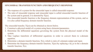
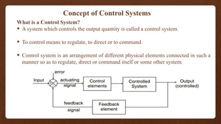
The document provides an overview of control systems, including definitions, classifications (linear vs non-linear, open loop vs closed loop), and key components like controllers and feedback mechanisms. It elaborates on various methodologies for modeling these systems mathematically, such as transfer functions and time response analysis. Additionally, it discusses the dynamic and static responses of mechanical systems, along with the electrical analogies used in their analysis.

1. CONTROL SYSTEMS
BY
G.V.SWATHI, ASST.PROF,EEE
ACE ENGINEERING COLLEGE
II B.TECH II SEM(R20 AUTONOMOUS)

2. Course
Outline
Modelling of Physical Systems
Time Response Analysis
Stability Analysis
Frequency Response Analysis
State Variable Analysis

3. Modelling of Physical Systems
UNIT-I

4. Concept of Control Systems
What is a Control System?
• A system which controls the output quantity is called a control system.
• To control means to regulate, to direct or to command.
• Control system is an arrangement of different physical elements connected in such a
manner so as to regulate, direct or command itself or some other system.

5. 1. Controlled Variable:
It is the quantity or condition that is measured & controlled.
2. Controller:
Controller means measuring the value of the controlled variable of the system & applying
the manipulated variable to the system to correct or to limit the deviation of the measured
value to the desired value.
3. Plant:
A plant is a piece of equipment, which is a set of machine parts functioning together. The
purpose of which is to perform a particular operation. Example: Furnace, Space craft etc.,
4. System:
A system is a combination of components that works together & performs certain
objective.

6. 5. Disturbance:
A disturbance is a signal that tends to affect the value of the output of a system. If a
disturbance is created inside the system, it is called internal. While an external
disturbance is generated outside the system.
6. Feedback Control:
It is an operation that, in the presence of disturbance tends to reduce the difference
between the output of a system & some reference input.
7. Servo Mechanism:
A servo mechanism is a feedback controlled system in which the output is some
mechanical position, velocity or acceleration

7. Classification of Control Systems
• Linear and Non Linear Systems
• Time Variant and Time Invariant Systems
• Continuous and Discrete Systems
• Dynamic and Static Systems
• Open Loop and Closed Loop Systems

8. Linear and Non Linear Systems
• In a linear system, the principle of superposition can be applied.
• In non- linear system, this principle can’t be applied .
• Therefore a linear system is that which obeys superposition principle &
homogeneity.
Examples of Linear System:
 Communication channels,
 A network that is solely resistive and has a steady DC source
 Filter circuits, and others.
Examples of Non-Linear System:
 An example of a non-linear system is the triangulation of GPS signals.
 A magnetization curve or the no load curve of a DC machine are well-known
examples of non-linear systems

9. Time Variant and Time Invariant Systems
• While operating a control system, if the parameters are unaffected by the time, then
the system is called Time Invariant Control System.
• Most physical systems have parameters changing with time.
• If this variation is measurable during the system operation then the system is called
Time Varying System.
• If there is no non-linearity in the time varying system, then the system may be called
as Linear Time varying System.

10. Continuous and Discrete Systems
Analog or Continuous System
• In these types of control systems, we have a continuous signal as the input to the
system. These signals are the continuous function of time.
Examples of continuous input signal
Sinusoidal type signal input source, square type of signal input source; the signal
may be in the form of continuous triangle etc.

11. Digital or Discrete System
In these types of control systems, we have a discrete signal (or signal may be in the form of pulse)
as the input to the system. These signals have a discrete interval of time.
Now there are various advantages of discrete or digital system over the analog system
 Digital systems can handle nonlinear control systems more effectively than the analog type
of systems.
 Power requirement in case of a discrete or digital system is less as compared to analog
systems.
 Reliability of the digital system is more as compared to an analog system. They also have a
small and compact size.
 Digital system works on the logical operations which increases their accuracy many times.
 Losses in case of discrete systems are less as compared to analog systems in general.

12. Dynamic and Static Systems
Dynamic Systems
• A system whose response or output depends upon the past or future inputs in addition
to the present input is called the dynamic system.
• The dynamic systems are also known as memory systems.
• Any continuous-time dynamic system can be described by a differential equation or
any discrete-time dynamic system by a difference equation.
Examples
An electric circuit containing inductors and (or) capacitors is an example of dynamic
system. Also, a summer or accumulator, a delay circuit, etc. are some examples of
discrete-time dynamic systems.

13. Static Systems
A system whose response or output is due to present input alone is known as static
system. The static system is also called the memoryless system.
Examples
A purely resistive electrical circuit is an example of static system

14. Open Loop and Closed Loop Systems
Open Loop Systems
• A system is said to be an open loop system when the system’s output has no effect on
the control action.
• In open loop system, the output is neither measured nor fed back for comparison
with the input.
• An open loop control system utilizes an actuating device (or controller) to control the
process directly

15. Advantages
• Simple and ease of maintenance
• Less expensive
• Stability is not a problem
• Convenient when output is hard to measure
Disadvantages
• Disturbances and changes in calibration cause errors
• Output may be different from what is desired

16. Exampl
es
• Washing Machine
• Electric Bulb
• Electric Hand Drier
• Time based Bread Toaster
• Automatic Water Faucet
• TV Remote Control
• Electric Clothes Drier
• Shades or Blinds on a window
• Stepper Motor or Servo Motor
• Inkjet Printers
• Door Lock System
• Traffic Control System

17. Closed Loop Systems
• A system that maintains a prescribed relationship between the output and the
reference input is called a closed-loop system or a feedback control system.
• The system uses a measurement of the output and feedback of the signal to compare
it with the desired output.
Feedback
Feedback control refers to an operation that, in the presence of disturbances, tends to
reduce the difference between the output of a system and some reference input and that
does so on the basis of this difference.

18. Advantages
• Can control for external factors
• More reliable and stable output
• Resilient to disturbances and changes
• More resource-efficient
Disadvantages
• More complex
• Requires tuning or integration
• Susceptible to oscillation or runaway conditions
• Sensor failure can cause unwanted system performance

19. • Automatic Electric Iron –Depending on the temperature of the iron heating
elements were controlled automatically.
• Servo Voltage Stabilizer – Stabilization in voltage is achieved by the feeding the
output voltage back to the system.
• Water Level Controller– Water level in the reservoirs decides the input water into
it.
• Air Conditioner –Air conditioner automatically adjusts its temperature depending
on its room temperature.
• In motor speed regulator using tachometer and/or current sensor , sensor senses the
speed and sends a feedback to the system to regulate its speed.
Exampl
es

22. Effect of Feedback
When feedback is given the error between system input and output is reduced. However
improvement of error is not only advantage. The effects of feedback are
1) Gain is reduced by a factor
2) Reduction of parameter variation by a factor 1 ± GH.
3) Improvement in sensitivity.
4) Stability may be affected.
5) Linearity of system improves
6) System Bandwidth increases

23. Open loop system Closed loop system
Any change in output has no effect on the
input. i.e., feedback does not exist
Changes in output, affects the input which is
possible by use of feedback.
Output is difficult to measure Output measurement is necessary
Feedback element is absent Feedback element is present
Error detector is absent Error detector is necessary
It is inaccurate and unreliable Highly accurate and reliable
Highly sensitive to the disturbance Less sensitive to the disturbances
Highly sensitive to the environmental
changes
Less sensitive to the environmental changes
Simple in construction and cheap Complicated to design and hence costly
System operation degenerates if the non-
linearities present
System operation degenerates if the non-
linearities present

24. Mathematical Modelling
• The set of mathematical equations, describing the dynamic characteristics of a
system is called Mathematical Modelling of the system.
• Most of the control systems are mechanical or electrical or both types of elements
and components.
• To analyze such systems , it is necessary to convert in mathematical models. This
can be done using
 Transfer function approach- applicable to linear time variant systems
 Steady state approach - non linear time varying systems and discreet systems

25. Transfer Function Modelling
The relationship between input and output of a system is given by the transfer function.
For a linear time−invariant system the response is separated into two parts : the forced
response and free response.
The forced response depends upon the initial values of input and the free response depends only on the initial
conditions on the output.
The transfer function P(s) of a continuous system is defined as

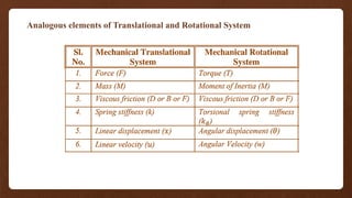
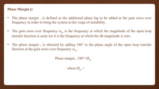
26. • The denominator is called the characteristic polynomial.
• The transform of the response may be rewritten as
Y(s) = P(s).U(s) + (terms due to all initial values)
• If all the initial conditions are assumed zero then
Y(s) = P(s) U(s)
• And the output as a function of time y(t) is simply
[P . U ] = y(t)

27. Definition
The transfer function is defined as the ratio of Laplace transform of output to Laplace
transform of input under assumption that all initial conditions are zero.
For example :
System g(t)
r(t) c(t)
r(t) = input
L r(t) = R(s)
c(t) = output
L c(t) = C(s)
g(t) = system function
Lg(t) = G(s)
∴ Transfer function G(s) :
G(s) =
G(s) =

28. Advantages of Transfer function
• If transfer function of a system is known, the response of the system to any input can
be determined very easily.
• A transfer function is a mathematical model and it gives the gain of the system.
• Since it involves the Laplace transform, the terms are simple algebraic expressions and
no differential terms are present.
• Poles and zeroes of a system can be determined from the knowledge of the transfer
function of the system.
Disadvantages of Transfer function
• Transfer function does not take into account the initial conditions.
• The transfer function can be defined for linear systems only.
• No inferences can be drawn about the physical structure of the system

29. Analysis of Mechanical Systems
In mechanical systems, motion can be of different types i.e. Translational, Rotational or
combination of both.
These systems are governed by Newton’s law of motion
Translational Systems
A system in which motion is taking place along straight line are Translational systems.
These systems are characterized by displacement, linear velocity and linear acceleration.
The following elements are dominantly involved in the analysis of translational motion
systems.
(i) Mass (ii) Spring (iii) Friction

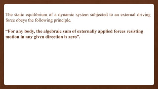
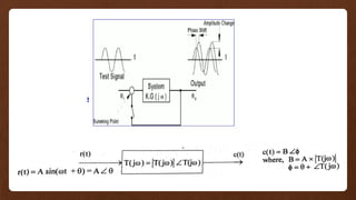
30. Mass
Taking Laplace transform
F(s) = M
A mass is denoted by M. If a force f is applied on it and it displays distance x, then
If a force f is applied on a mass M and it displays distance x1in the direction of f and
distance x2 in the opposite direction, then
Taking Laplace transform
F(s) = M ]

31. Linear Spring
A spring is denoted by K. If a force f is applied on it and it displays distance x, then
f = Kx
Taking Laplace transform
F(s) = K X(s)
If a force f is applied on a spring K and it displays distance x1in the direction of f and
distance x2 in the opposite direction, then
f = K()
Taking Laplace transform
F(s) = K X1(s) – X2(s)

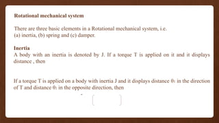
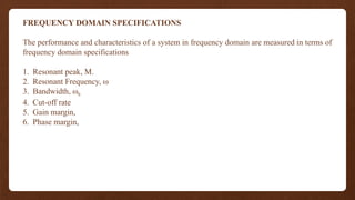
32. Friction
A damper is denoted by B. If a force f is applied on it and it displays distance x, then
f = B
Taking Laplace transform
F(s) = B s X(s)
If a force f is applied on a damper B and it displays distance x1in the direction of f and
distance x2 in the opposite direction, then
f = B[ - ]
Taking Laplace transform
F(s) = B s [X1(s) – X2(s)]

33. Rotational System

34. Analogous elements of Translational and Rotational System

35. The static equilibrium of a dynamic system subjected to an external driving
force obeys the following principle,
“For any body, the algebraic sum of externally applied forces resisting
motion in any given direction is zero”.

36. Rotational mechanical system
There are three basic elements in a Rotational mechanical system, i.e.
(a) inertia, (b) spring and (c) damper.
Inertia
A body with an inertia is denoted by J. If a torque T is applied on it and it displays
distance , then
If a torque T is applied on a body with inertia J and it displays distance θ1 in the direction
of T and distance θ2 in the opposite direction, then
-

37. Spring
A spring is denoted by K. If a torque T is applied on it and it displays distance θ, then
T =Kθ.
If a torque T is applied on a body with inertia J and it displays distance θ1 in the direction
of T and distance θ2 in the opposite direction, then
T = K θ1- θ2
Damper
A damper is denoted by D. If a torque T is applied on it and it displays distance θ, then
T = D
If a torque T is applied on a body with inertia J and it displays distance θ1 in the
direction of T and distance θ2 in the opposite direction , then
T = D -

38. Electrical Analogous of Mechanical Translational systems
• Two systems are said to be analogous to each other if the following two conditions
are satisfied.
 The two systems are physically different.
 Differential equation modelling of those two systems are same.
• Electrical systems and mechanical systems are two physically different systems.
• There are two types of electrical analogies of translational mechanical systems.
Those are
Force Voltage analogy and Force Current analogy.

39. Force Voltage Analogy
In force voltage analogy, the mathematical equations of translational mechanical system
are compared with mesh equations of the electrical system.
Consider the following translational mechanical system shown in the following figure.
F=Fm+ Fb+ Fk
+ B

40. • Consider the electrical system consists of a resistor, an inductor and a capacitor.
• All these electrical elements are connected in a series.
• The input voltage applied to this circuit is V volts and the current flowing through
the circuit is i amps.
V
Substitute, then (2)

41. Comparing equations ( 1) and (2)
Translational Mechanical System Electrical System
Force(F) Voltage(V)
Mass(M) Inductance(L)
Frictional Coefficient(B) Resistance(R)
Spring Constant(K) Reciprocal of Capacitance (1/C)
Displacement(x) Charge(q)
Velocity(v) Current(i)

42. Force Current Analogy
• In force current analogy, the mathematical equations of the translational mechanical
system are compared with the nodal equations of the electrical system.
• Consider the electrical system consists of current source, resistor, inductor and
capacitor.
• All these electrical elements are connected in parallel.
(3)
Substitute, then
+ (4)

43. Comparing equations ( 3) and (4)
Translational Mechanical System Electrical System
Force(F) Current(i)
Mass(M) Capacitance(C)
Frictional coefficient(B) Reciprocal of Resistance(1/R)
Spring constant(K) Reciprocal of Inductance(1/L)
Displacement(x) Magnetic Flux(Ø)
Velocity(v) Voltage(V)

44. BLOCK DIAGRAM REDUCTION
• In order to draw the block diagram of a practical system each element of practical
system is represented by a block.
• For a closed loop system, the function of comparing the different signals is indicated
by the summing point while a point from which signal is taken for the feedback
purpose is indicated by take off point in block diagrams.
• A block diagram has following five basic elements associated with it.
1) Functional Blocks
2) Transfer functions of elements shown inside the functional blocks
3) Summing points
4) Take off points
5) Arrow

45. Transfer function of a Closed Loop System

47. Rules for Block Diagram Reduction
Rule 1 : Associative Law
Now even though we change the position of the two summing points, output remains
same
Thus associative law holds good for summing points which are directly connected to each
other.

48. Rule 2:
Here G1 and G2 are in series and can be combined. But because of the take off point
G3 cannot be combined.

49. Time Response Analysis
UNIT-II

50. Time Response
 In time domain analysis, time is the independent variable. When a system is
given an excitation, there is a response (output).
 Definition: Theresponse of a system to an applied excitation
is called “Time Response” and it is a function of c(t).
 Time Response – Example
The response of motor’s speed when a command is given to increase the speed is shown
in figure,
As seen from figure, the motors speed gradually picks up from 1000 rpm and moves towards 1500 rpm. It
overshoots and again corrects itself and finally settles down at the last value
3

51. Generally speaking, the response of any system thus has two parts
 Transient Response
 Steady State Response
• That part of the time response that goes to zero as time becomes very large is called
as “Transient Response”
i.e.
• As the name suggests that transient response remains only for some time from
initial state to final state.
L c ( t ) 
0
t  

52. 4
From the transient response we can know;
 When system begins to respond after an input is given.
 How much time it takes to reach the output for the first time.
 Whether the output shoots beyond the desired value & how much.
 Whether the output oscillates about its final value.
 When does it settle to the final value.
• That part of the response that remains after the transients have died out is called
“Steady State Response”.
From the steady state we can know;
 How long it took before steady state was reached.
Whether there is any error between the desired and actual values.
Whether this error is constant, zero or infinite i.e. unable to track the input.

53. Shadab. A. Siddique

54. Standard Test Signal
• It is very interesting fact to know that most control systems do not know what
their inputs are going to be.
• Thus system design cannot be done from input point of view as we are unable to
know in advance the type input.
Need of Standard Test Signal
 From example;
When a radar tracks an enemy plane the nature of the enemy plane’s variation
is random.
 The terrain, curves on road etc. are random for a drives in an automobile system.
The loading on a shearing machine when and which load will be applied or
thrown of.

55. Thus from such types of inputs we can expect a system in general to get an input
which may be;
a) A sudden change
b) A momentary shock
c) A constant velocity
d) A constant acceleration
Hence these signals form standard test signals. The response to these
signals is analyzed. The above inputs are called as,
a) Step input - Signifies a sudden change
b) Impulse input – Signifies momentary shock
c) Ramp input – Signifies a constant velocity
d) Parabolic input – Signifies constant acceleration
Shadab. A. Siddique

56. Standard Test Signal
Step Input
Mathematical Representations
r(t) = R. u(t)
= 0
Graphical Representations
t>0
t<0
Shadab. A. Siddique
This signal signifies a sudden change in the reference input r(t) at time t=0
Laplace Representations L =

57. Unit Step Input
Mathematical Représentations
r(t) = 1. u(t)
= 0
t>0
t<0
Graphical Representations
This signal signifies a sudden change in the reference input r(t) at time t=0
Laplace Representations L =

58. Ramp Input
Mathematical Representations
r(t) = R.t
= 0
t>0
t<0
Graphical Representations
Signal have constant velocity i.e. constant change in it’s value w.r.t. time
Laplace Representations L =
Ramp signal is integral of step signal.

59. Unit Ramp Input
Mathematical Representations
r(t) = 1. t
= 0
t>0
t<0
Graphical Representations
Laplace Representations L =

60. Parabolic Input
Mathematical Representations
r(t) = R.
= 0
t>0
t<0
Graphical Representations
Laplace Representations L =
Parabolic input is integral of ramp input.

61. Impulse Input
r(t) = =1
= 0
t>0
t<0
Graphical Representations
Mathematical Representations
The function has a unit value only for t=0.
In practical cases, a pulse whose time approaches zero is taken as an impulse function.
Laplace Representations L = 1

62. SINUSOIDAL TRANSFER FUNCTION AND FREQUENCY RESPONSE
• The response of a system for the sinusoidal input is called sinusoidal response.
• The ratio of sinusoidal response and sinusoidal input is called sinusoidal transfer function of
the system and in general, it is denoted by T(jω).
• The sinusoidal transfer function is the frequency domain representation of the system, and so
it is also called frequency domain transfer function.
The sinusoidal transfer, T(jω) can be obtained as shown below.
1. Construct a physical model of a system using basic elements/parameters.
2. Determine the differential equations governing the system from the physical model of the
system.
3. Take Laplace transform of differential equations in order to convert them to s-domain
equation.
4. Determine s-domain transfer function, T(s), which is ratio of s-domain output and input.
5. Determine the frequency domain transfer function, T(jω) by replacing s by jo in the s-domain
transfer function, T(s).

63. If the s-domain transfer function, T(s) is known, then frequency domain transfer
function, T(jω) can be obtained directly from T(s) by replacing s by jω.
i.e., T(s) T(jω)
s= jω

64. • Consider a linear time invariant system with frequency domain transfer function, T(jω).
• Let the system be excited by a sinusoidal signal frequency ω, amplitude A, and phase θ.
• Now the response or output will also be a sinusoidal signal of same frequency ω, but
the amplitude and phase of response will be modified by amplitude and phase of the
transfer function respectively.
• Now, the amplitude of the response is given by the product of the amplitude of the input
and transfer function. The phase of the response is given by the sum of the phase of the
input and transfer junction.
• The frequency response can be evaluated for open loop system and closed loop system.
• The frequency domain transfer function of open loop and closed loop systems can be
obtained from the s-domain transfer function by replacing s by jω.

66. The advantages of frequency response analysis are the following.
1. The absolute and relative stability of the closed loop system can be estimated from the
knowledge of their open loop frequency response.
2. The practical testing of systems can be easily carried with available sinusoidal signal
generators and precise measurement equipment’s.
3. The transfer function of complicated systems can be determined experimentally by frequency
response tests.
4. The design and parameter adjustment of the open loop transfer function of a system for
specified closed loop performance is carried out more easily in frequency domain.
5. When the system is designed by use of the frequency response analysis, the effects of noise
disturbance and parameters variations are relatively easy to visualize and incorporate corrective
measures.
6. The frequency response analysis and designs can be extended to certain nonlinear control
systems.

67. FREQUENCY DOMAIN SPECIFICATIONS
The performance and characteristics of a system in frequency domain are measured in terms of
frequency domain specifications
1. Resonant peak, M.
2. Resonant Frequency, ω
3. Bandwidth, ωb
4. Cut-off rate
5. Gain margin,
6. Phase margin,

68. Resonant Peak (M): The maximum value of the magnitude of closed loop transfer function is
called the resonant peak, M. A large resonant peak corresponds to a large overshoot in transient
response.
Resonant Frequency (ω): The frequency at which the resonant peak occurs is called resonant
frequency, w, This is related to the frequency of oscillation in the step response and thus it is
indicative of the speed of transient response.
Bandwidth (ωb): The Bandwidth is the range of frequencies for which the system normalized
gain is more than -3 db. The frequency at which the gain is -3 db is called cut-off frequency.
Bandwidth is usually defined for closed loop system and it transmits the signals whose
frequencies are less than the cut-off frequency. The Bandwidth is a measure of the ability of a
feedback system to reproduce the input signal, noise rejection characteristics and rise time. A large
bandwidth corresponds to a small rise time or fast response.
Cut-off Rate: The slope of the log-magnitude curve near the cut off frequency is called cut-off
rate. The cut -off rate indicates the ability of the system to distinguish the signal from noise

69. Gain Margin :
• The gain margin, is defined as the value of gain, to be added to system, in order to bring the
system to the verge of instability.
• The gain margin, is given by the reciprocal of the magnitude of open loop transfer function at
phase cross over frequency.
• The frequency at which the phase of open loop transfer function is 180° is called the phase
cross-over frequency, ωpc .
Gain Margin, =
The gain margin in db can be expressed as,
in db = 20 log = 20 log

70. Phase Margin ()
• The phase margin , is defined as the additional phase lag to be added at the gain cross over
frequency in order to bring the system to the verge of instability.
• The gain cross over frequency ωgc is the frequency at which the magnitude of the open loop
transfer function is unity (or it is the frequency at which the db magnitude is zero.
• The phase margin , is obtained by adding 180° to the phase angle of the open loop transfer
function at the gain cross over frequency ωgc .
Phase margin , 180°+Øgc
where Øgc =

71. Frequency Response Plots

72. • Frequency response analysis of control systems can be carried either analytically or graphically.
The various graphical techniques available for frequency response analysis are,
1. Bode plot
2. M and N circles
3. Nichols chart
4. Nichols plot
• The Bode plot, Polar plot and Nichols plot are usually drawn for open loop systems.
• From the open loop response plot the performance and stability of closed loop system are
estimated.
• The M and N circles and Nichols chart are used to graphically determine the frequency response
of unity feedback closed loop system from the knowledge of open loop response.
• The frequency response plots are used to determine the frequency domain specifications, to study
the stability of the systems and to adjust the gain of the system to satisfy the desired
specifications.

73. BODE PLOT
• The Bode plot is a frequency response plot of the sinusoidal transfer function of a system.
• A Bode plot consists of two graphs. One is a plot of the magnitude of a sinusoidal transfer
function versus log ω. The other is a plot of the phase angle of a sinusoidal transfer function
versus log ω.
• The Bode plot can be drawn for both open loop and closed loop system. Usually the bode plot is
drawn for open loop system.
• The standard representation of the logarithmic magnitude of open loop transfer function of
G(jω) is 20 log| G(jω) | where the base of the logarithm is 10. The unit used in this
representation of the magnitude is the decibel, usually abbreviated db. The curves are drawn on
semilog paper, using the log scale (abcissa) for frequency and the linear scale (ordinate for
either magnitude (in decibels) or phase angle (in degrees).
• The main advantage of the bode plot is that multiplication of magnitudes can be converted into
addition.

74. Consider the open loop transfer function, G(s) =
G(jω) =
=
The magnitude of G(jω) = | G(jω) | =
The phase angle of the G(jω) = G(jω) = -
The magnitude of G(jω) in decibels is
| G(jω) | in db = 20 log | G(jω) |
= 20 log

75. = 20 log
= 20log + 20log + 20 log +20 log
= 20log + 20log - 20 log - 20 log
From the equation, when the magnitude is expressed in db, the multiplication is converted to
addition.
• Hence in magnitude plot, the db magnitudes of individual factors of G(jω) can be added.
• Therefore to sketch the magnitude plot, a knowledge of the magnitude variations of individual
factor is essential.

76. Basic factor of G(jω)
1. Constant gain, K
2. Integral factor, or
3. Derivative factor, K or K
4. First order factor in denominator, or
5. First order factor in numerator, or

77. Constant gain, K

78. Integral factor, or

80. Derivative factor, K or K

82. First order factor in denominator, or

84. First order factor in numerator, or