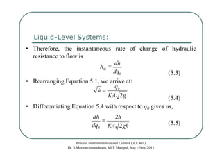
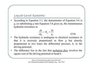
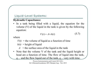
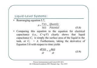
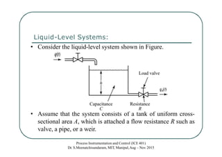
The document discusses mathematical modeling of liquid-level systems, focusing on fluid flow principles, such as laminar and turbulent flow, and their representation through differential equations. It introduces concepts of hydraulic resistance and capacitance in liquid systems, explaining how these can be modeled and analyzed for dynamic characteristics. The document also outlines example calculations and assignments related to hydraulic systems behavior over time.

![Liquid-Level Systems:
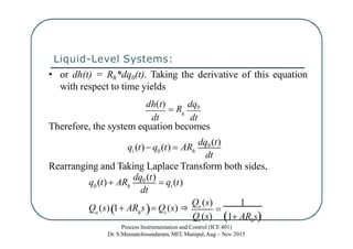
RAs 1H(s) RQi (s)
Qi (s) RAs 1
Qi (s)
Process Instrumentation and Control (ICE 401)
Dr. S.Meenatchisundaram, MIT, Manipal,Aug – Nov 2015
RAs 1 0
R
Q (s)
H(s)
(5.15)
• where,
H(s) = L[h(t)] and Qi(s) = L[qi(t)]
• Rearranging eqn. 5.15,
H (s)
R
(5.16)
• If however, q0 is taken as the output, the input being the
same, then the transfer function is
Q0 (s)
1
(5.17)](https://image.slidesharecdn.com/class7-mathematicalmodelingofliquid-levelsystems-150825045422-lva1-app68911-240707111711-24d2ad8a/85/mathematical-modeling-of-liquid-level-systems-13-320.jpg)