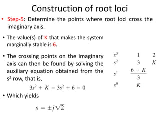
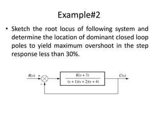
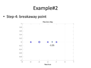
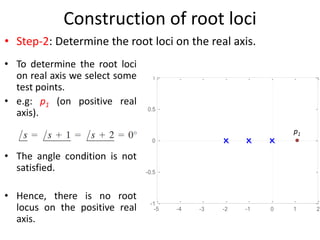
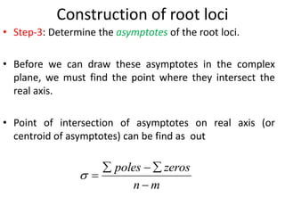
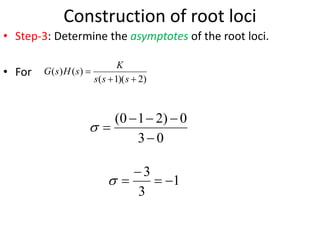
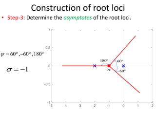
The document outlines the steps for constructing root loci in control systems, detailing methods to locate poles and zeros in the s-plane, determine asymptotes, breakaway and break-in points, and identify points crossing the imaginary axis. It provides examples of calculating the required parameters for unity feedback systems and illustrates various techniques such as the Routh stability criterion. Additionally, it includes several homework problems to reinforce the concepts discussed.

1. Control Systems (CS)
Dr. Imtiaz Hussain
Associate Professor
Mehran University of Engineering & Technology Jamshoro, Pakistan
email: imtiaz.hussain@faculty.muet.edu.pk
URL :http://imtiazhussainkalwar.weebly.com/
Lecture-23-24
Construction of Root Loci
1

2. Construction of root loci
• Step-1: The first step in constructing a root-locus plot
is to locate the open-loop poles and zeros in s-plane.
)
2
)(
1
(
)
(
)
(



s
s
s
K
s
H
s
G
-5 -4 -3 -2 -1 0 1 2
-1
-0.5
0
0.5
1
Pole-Zero Map
Real Axis
Imaginary
Axis

3. -5 -4 -3 -2 -1 0 1 2
-1
-0.5
0
0.5
1
Pole-Zero Map
Real Axis
Imaginary
Axis
Construction of root loci
• Step-2: Determine the root loci on the real axis.
p1
• To determine the root loci
on real axis we select some
test points.
• e.g: p1 (on positive real
axis).
• The angle condition is not
satisfied.
• Hence, there is no root
locus on the positive real
axis.

4. -5 -4 -3 -2 -1 0 1 2
-1
-0.5
0
0.5
1
Pole-Zero Map
Real Axis
Imaginary
Axis
Construction of root loci
• Step-2: Determine the root loci on the real axis.
p2
• Next, select a test point on the
negative real axis between 0 and
–1.
• Then
• Thus
• The angle condition is satisfied.
Therefore, the portion of the
negative real axis between 0 and
–1 forms a portion of the root
locus.

5. -5 -4 -3 -2 -1 0 1 2
-1
-0.5
0
0.5
1
Pole-Zero Map
Real Axis
Imaginary
Axis
Construction of root loci
• Step-2: Determine the root loci on the real axis.
p3
• Now, select a test point on the
negative real axis between -1 and
–2.
• Then
• Thus
• The angle condition is not
satisfied. Therefore, the negative
real axis between -1 and –2 is not
a part of the root locus.

6. -5 -4 -3 -2 -1 0 1 2
-1
-0.5
0
0.5
1
Pole-Zero Map
Real Axis
Imaginary
Axis
Construction of root loci
• Step-2: Determine the root loci on the real axis.
p4
• Similarly, test point on the
negative real axis between -2
and – ∞ satisfies the angle
condition.
• Therefore, the negative real
axis between -2 and – ∞ is part
of the root locus.

7. -5 -4 -3 -2 -1 0 1 2
-1
-0.5
0
0.5
1
Pole-Zero Map
Imaginary
Axis Construction of root loci
• Step-2: Determine the root loci on the real axis.

8. Construction of root loci
• Step-3: Determine the asymptotes of the root loci.
• where
• n-----> number of poles
• m-----> number of zeros
• For this Transfer Function
m
n
k
asymptotes
of
Angle






)
1
2
(
180

)
2
)(
1
(
)
(
)
(



s
s
s
K
s
H
s
G
0
3
)
1
2
(
180





k


9. Construction of root loci
• Step-3: Determine the asymptotes of the root loci.
• Since the angle repeats itself as k is varied, the distinct angles
for the asymptotes are determined as 60°, –60°, -180°and
180°.
• Thus, there are three asymptotes having angles 60°, –60°,
180°.
3
when
420
2
when
300
1
when
180
0
n
whe
60
















k
k
k
k


10. Construction of root loci
• Step-3: Determine the asymptotes of the root loci.
• Before we can draw these asymptotes in the complex
plane, we must find the point where they intersect the
real axis.
• Point of intersection of asymptotes on real axis (or
centroid of asymptotes) can be find as out
m
n
zeros
poles







11. Construction of root loci
• Step-3: Determine the asymptotes of the root loci.
• For
0
3
0
)
2
1
0
(






)
2
)(
1
(
)
(
)
(



s
s
s
K
s
H
s
G
1
3
3






12. Construction of root loci
• Step-3: Determine the asymptotes of the root loci.
-5 -4 -3 -2 -1 0 1 2
-1
-0.5
0
0.5
1
Pole-Zero Map
Real Axis
Imaginary
Axis


60

 60

180




 180
,
60
,
60

1




13. Home Work
• Consider following unity feedback system.
• Determine
– Root loci on real axis
– Angle of asymptotes
– Centroid of asymptotes

14. Construction of root loci
• Step-4: Determine the breakaway point.
• The breakaway point
corresponds to a point
in the s plane where
multiple roots of the
characteristic equation
occur.
• It is the point from
which the root locus
branches leaves real
axis and enter in
complex plane. -5 -4 -3 -2 -1 0 1 2
-1
-0.5
0
0.5
1
Pole-Zero Map
Real Axis
Imaginary
Axis

15. Construction of root loci
• Step-4: Determine the break-in point.
• The break-in point
corresponds to a point
in the s plane where
multiple roots of the
characteristic equation
occur.
• It is the point where the
root locus branches
arrives at real axis.
-5 -4 -3 -2 -1 0 1 2
-1
-0.5
0
0.5
1
Pole-Zero Map
Real Axis
Imaginary
Axis

16. Construction of root loci
• Step-4: Determine the breakaway point or break-in point.
• The breakaway or break-in points can be determined from the
roots of
• It should be noted that not all the solutions of dK/ds=0
correspond to actual breakaway points.
• If a point at which dK/ds=0 is on a root locus, it is an actual
breakaway or break-in point.
• Stated differently, if at a point at which dK/ds=0 the value of K
takes a real positive value, then that point is an actual breakaway
or break-in point.
0

ds
dK

17. Construction of root loci
• Step-4: Determine the breakaway point or break-in point.
• The characteristic equation of the system is
• The breakaway point can now be determined as
)
2
)(
1
(
)
(
)
(



s
s
s
K
s
H
s
G
0
)
2
)(
1
(
1
)
(
)
(
1 





s
s
s
K
s
H
s
G
1
)
2
)(
1
(



 s
s
s
K
 
)
2
)(
1
( 


 s
s
s
K
 
)
2
)(
1
( 


 s
s
s
ds
d
ds
dK

18. Construction of root loci
• Step-4: Determine the breakaway point or break-in point.
• Set dK/ds=0 in order to determine breakaway point.
 
)
2
)(
1
( 


 s
s
s
ds
d
ds
dK
 
s
s
s
ds
d
ds
dK
2
3 2
3




2
6
3 2



 s
s
ds
dK
0
2
6
3 2



 s
s
0
2
6
3 2


 s
s
5774
.
1
4226
.
0




s

19. Construction of root loci
• Step-4: Determine the breakaway point or break-in point.
• Since the breakaway point must lie on a root locus between 0
and –1, it is clear that s=–0.4226 corresponds to the actual
breakaway point.
• Point s=–1.5774 is not on the root locus. Hence, this point is
not an actual breakaway or break-in point.
• In fact, evaluation of the values of K corresponding to s=–
0.4226 and s=–1.5774 yields
5774
.
1
4226
.
0




s

20. Construction of root loci
• Step-4: Determine the breakaway point.
-5 -4 -3 -2 -1 0 1 2
-1
-0.5
0
0.5
1
Pole-Zero Map
Real Axis
Imaginary
Axis


60

 60

180
4226
.
0


s

21. Construction of root loci
• Step-4: Determine the breakaway point.
4226
.
0


s
-5 -4 -3 -2 -1 0 1 2
-1
-0.5
0
0.5
1
Pole-Zero Map
Real Axis
Imaginary
Axis

22. Home Work
• Determine the Breakaway and break in points

23. Solution
• Differentiating K with respect to s and setting the derivative equal to zero yields;
Hence, solving for s, we find the
break-away and break-in points; s = -1.45 and 3.82
1
2
3
)
15
8
(
2
2






s
s
s
s
K
)
15
8
(
)
2
3
(
2
2






s
s
s
s
K
0
)
15
8
(
)]
8
2
)(
2
3
(
)
3
2
)(
15
8
[(
2
2
2
2












s
s
s
s
s
s
s
s
ds
dK
0
61
26
11 2


 s
s

24. Construction of root loci
• Step-5: Determine the points where root loci cross the
imaginary axis.
-5 -4 -3 -2 -1 0 1 2
-1
-0.5
0
0.5
1
Pole-Zero Map
Imaginary
Axis


60

 60

180

25. Construction of root loci
• Step-5: Determine the points where root loci cross the
imaginary axis.
– These points can be found by use of Routh’s stability criterion.
– Since the characteristic equation for the present system is
– The Routh Array Becomes

26. Construction of root loci
• Step-5: Determine the points where root loci cross the
imaginary axis.
• The value(s) of K that makes the system
marginally stable is 6.
• The crossing points on the imaginary
axis can then be found by solving the
auxiliary equation obtained from the
s2 row, that is,
• Which yields

27. Construction of root loci
• Step-5: Determine the points where root loci cross the
imaginary axis.
• An alternative approach is to let s=jω in the characteristic
equation, equate both the real part and the imaginary part to
zero, and then solve for ω and K.
• For present system the characteristic equation is
0
2
3 2
3



 K
s
s
s
0
2
)
(
3
)
( 2
3



 K
j
j
j 


0
)
2
(
)
3
( 3
2



 

 j
K

28. Construction of root loci
• Step-5: Determine the points where root loci cross the
imaginary axis.
• Equating both real and imaginary parts of this equation
to zero
• Which yields
0
)
2
(
)
3
( 3
2



 

 j
K
0
)
3
( 2

 
K
0
)
2
( 3




30. -7 -6 -5 -4 -3 -2 -1 0 1 2
-5
-4
-3
-2
-1
0
1
2
3
4
5
Root Locus
Real Axis
Imaginary
Axis

31. Example#1
• Consider following unity feedback system.
• Determine the value of K such that the damping ratio of
a pair of dominant complex-conjugate closed-loop poles
is 0.5.
)
2
)(
1
(
)
(
)
(



s
s
s
K
s
H
s
G

32. Example#1
• The damping ratio of 0.5 corresponds to

 cos


 1
cos



 
60
)
5
.
0
(
cos 1


33. ?

34. Example#1
• The value of K that yields such poles is found from the
magnitude condition
1
)
2
)(
1
( 5780
.
0
3337
.
0


 

 j
s
s
s
s
K

36. Example#1
• The third closed loop pole at K=1.0383 can be obtained
as
0
)
2
)(
1
(
1
)
(
)
(
1 





s
s
s
K
s
H
s
G
0
)
2
)(
1
(
0383
.
1
1 



s
s
s
0
0383
.
1
)
2
)(
1
( 


 s
s
s

38. Home Work
• Consider following unity feedback system.
• Determine the value of K such that the natural
undamped frequency of dominant complex-conjugate
closed-loop poles is 1 rad/sec.
)
2
)(
1
(
)
(
)
(



s
s
s
K
s
H
s
G

39. -3 -2.5 -2 -1.5 -1 -0.5 0 0.5 1 1.5
-2
-1.5
-1
-0.5
0
0.5
1
1.5
2
Root Locus
Imaginary
Axis
-0.2+j0.96

40. Example#2
• Sketch the root locus of following system and
determine the location of dominant closed loop
poles to yield maximum overshoot in the step
response less than 30%.

41. Example#2
• Step-1: Pole-Zero Map
-5 -4 -3 -2 -1 0 1
-1
-0.8
-0.6
-0.4
-0.2
0
0.2
0.4
0.6
0.8
1
Pole-Zero Map
Real Axis
Imaginary
Axis

42. Example#2
• Step-2: Root Loci on Real axis
-5 -4 -3 -2 -1 0 1
-1
-0.8
-0.6
-0.4
-0.2
0
0.2
0.4
0.6
0.8
1
Pole-Zero Map
Real Axis
Imaginary
Axis

43. Example#2
• Step-3: Asymptotes
-5 -4 -3 -2 -1 0 1
-1
-0.8
-0.6
-0.4
-0.2
0
0.2
0.4
0.6
0.8
1
Pole-Zero Map
Real Axis
Imaginary
Axis


 90

2




44. Example#2
• Step-4: breakaway point
-5 -4 -3 -2 -1 0 1
-1
-0.8
-0.6
-0.4
-0.2
0
0.2
0.4
0.6
0.8
1
Pole-Zero Map
Real Axis
Imaginary
Axis
-1.55

45. Example#2
-4.5 -4 -3.5 -3 -2.5 -2 -1.5 -1 -0.5 0 0.5
-8
-6
-4
-2
0
2
4
6
8
Root Locus
Real Axis
Imaginary
Axis

46. Example#2
• Mp<30% corresponds to
100
2
1

 



e
M p
100
%
30
2
1

 



e
35
.
0



47. Example#2
-4.5 -4 -3.5 -3 -2.5 -2 -1.5 -1 -0.5 0 0.5
-8
-6
-4
-2
0
2
4
6
8
0.35
0.35
6
6
Root Locus
Real Axis
Imaginary
Axis

48. Example#2
-4.5 -4 -3.5 -3 -2.5 -2 -1.5 -1 -0.5 0 0.5
-8
-6
-4
-2
0
2
4
6
8
0.35
0.35
6
6
System: sys
Gain: 28.9
Pole: -1.96 + 5.19i
Damping: 0.354
Overshoot (%): 30.5
Frequency (rad/sec): 5.55
Root Locus
Real Axis
Imaginary
Axis

49. END OF LECTURES-23-24
To download this lecture visit
http://imtiazhussainkalwar.weebly.com/