Download to read offline

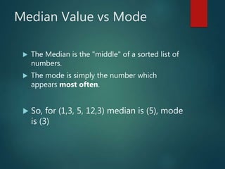

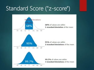
![A Practical Example
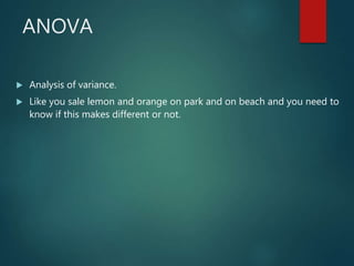
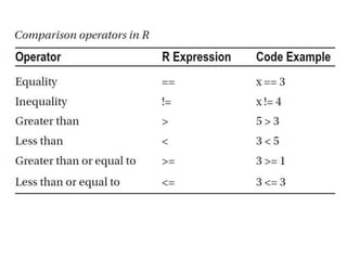
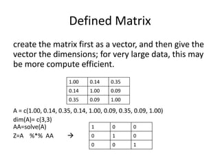
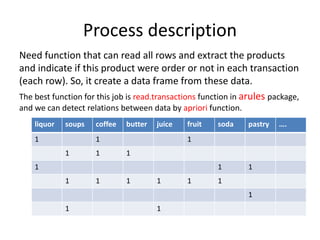
Your company packages sugar in 1 kg bags.
When you weigh a sample of bags you get these results:
1007g, 1032g, 1002g, 983g, 1004g, ... (a hundred measurements)
Mean = 1010g
Standard Deviation = 20g
How many package less that 1 KG? 30.85%
How to fix this problem?
Let's adjust the machine so that 1000g is:
at −3 standard deviations: 0.1%
at −2.5 standard deviations: 0.6% [Good choice]
The standard deviation is 20g, and we need 2.5 of them: 2.5 × 20g = 50g, so
increase the package 50 gram when weight to fix the problem.](https://image.slidesharecdn.com/r-201118205115/85/R-for-Statistical-Computing-14-320.jpg)

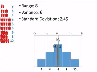
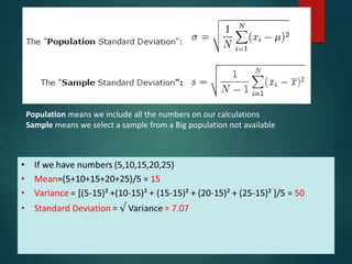
![Some R’s operations
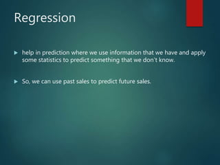
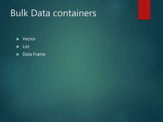
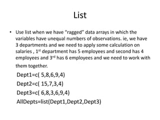
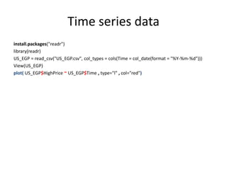
X=5
Y=4
Z=x*y
A=1:10 1,2,3,4,5,6,7,8,9,10
B=A^2 1,4,9,16,25,36,49,64,81,100
K=B[1:5] 1,4,9,16,25
A[1:3]=c(33,66,99)
A 33,66,99,4,5,6,7,8,9,10](https://image.slidesharecdn.com/r-201118205115/85/R-for-Statistical-Computing-23-320.jpg)
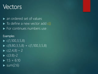
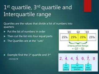
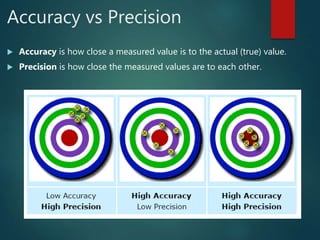
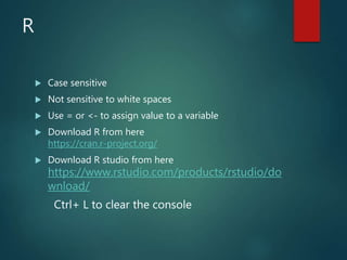
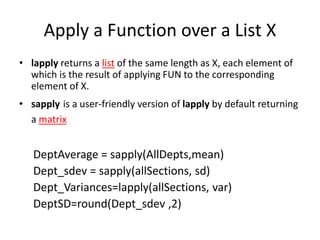
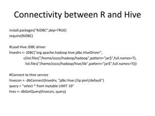
![Set title to the vector
X=100:102
names(X)=c(“First”,”Second”,”Third”)
X
Y=1:26
names(Y)=toupper(letters[1:26])
First Second Third
100 101 102
A B C D E F G H I J K …
1 2 3 4 5 6 7 8 9 10 11 ..](https://image.slidesharecdn.com/r-201118205115/85/R-for-Statistical-Computing-26-320.jpg)
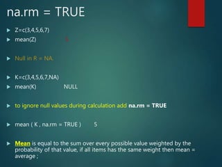
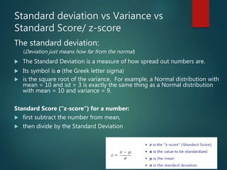
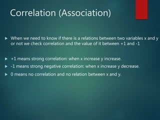
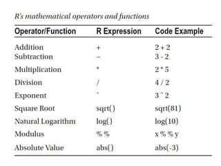
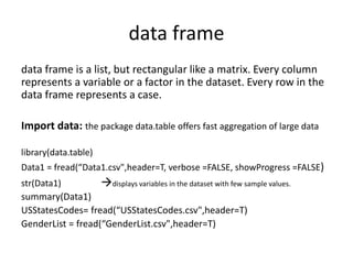
![List
Each element of the list can has different type.
Example
zz= list(1,6,’ssss’,true)
kk= list (first=1,second=6,third=‘ssss’,fourth=true)
// kk[1:3] // kk[1] // kk[“first”] // kk$first
To convert vector to list use as.list(vector name)
To convert list to vector use as.numeric(list name) or unlist(list name)](https://image.slidesharecdn.com/r-201118205115/85/R-for-Statistical-Computing-29-320.jpg)

![Data Frame
It is like a DB table contains rows and columns
To create it use data.frame()
Example
zz=data.frame( x=c(1:5) , y=letters[1:5] )
Related Functions
rownames, colnames,dim , dimnames, nrow, ncol](https://image.slidesharecdn.com/r-201118205115/85/R-for-Statistical-Computing-31-320.jpg)

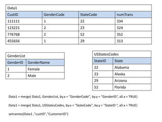
![Data1
CustomerID Gender Code Gender Name State Code State numTrans
111111 1 Female 22 Alabama 334
123221 2 male 23 Alaska 324
776768 2 male 52 Florida 352
455656 1 Female 29 Arizona 313
Select data that met one criteria
which (Data1 $ GenderCode = 2)
Select some columns from data
SelectedColumnsNames= c(“CustomerID” , ”numTrans”)
Data2 = Data1[SelectedColumnsNames]
Get Information about column
summary(Data1 $ numTrans)
Min. 1st Qu. Median Mean 3rd Qu. Max.
313 333 350 366 377 400](https://image.slidesharecdn.com/r-201118205115/85/R-for-Statistical-Computing-41-320.jpg)

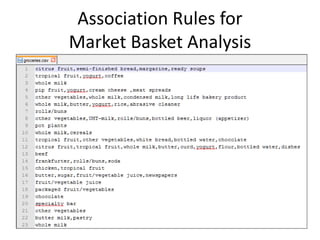
![Steps
Install.packages (“arules”)
require(arules)
setwd("C:/R-datasets")
SalesData =read.transactions(“groceries.csv”, sep=“ , ”)
View data
str(SalesData)
summary(SalesData) get calculation information about data
inspect(SalesData[1:3]) read sales transactions that exists in 1st 3 rows
itemFrequency(SalesData[,1]) all rows and product number 1
itemFrequency(SalesData [ , 1 : 6 ] ) all rows and products from 1 to 6
Plot
itemFrequencyPlot (SalesData , support = 0.05) draw items that exceed a limit 5%
itemFrequencyPlot (SalesData , topN = 20) draw top 20 sales items
Detect Association
AssociationRules1 =
apriori (SalesData, parameter = list (support = 0.007,confidence=0.25, minlen=2))](https://image.slidesharecdn.com/r-201118205115/85/R-for-Statistical-Computing-47-320.jpg)
![Browse Association rules
• Inspect(AssociationRules1 [1:2] )
• Inspect(sort(AssociationRules1, by=“lift”)[1:4])
Lift is simply the ratio of these values: target
response divided by average response.
LHS RHS Support Confidence Lift
Coffee Milk 0.006 0.44 4.2](https://image.slidesharecdn.com/r-201118205115/85/R-for-Statistical-Computing-48-320.jpg)

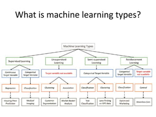
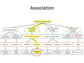
This document provides an overview of statistical concepts and analysis techniques in R, including measures of central tendency, data variability, correlation, regression, and time series analysis. Key points covered include mean, median, mode, variance, standard deviation, z-scores, quartiles, standard deviation vs variance, correlation, ANOVA, and importing/working with different data structures in R like vectors, lists, matrices, and data frames.