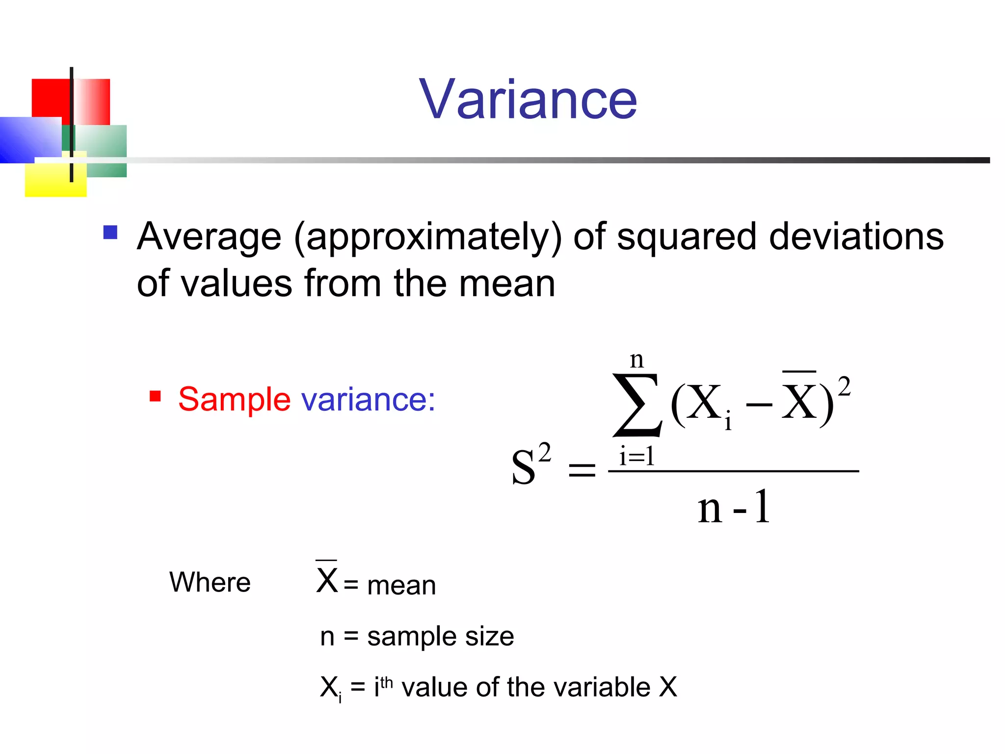
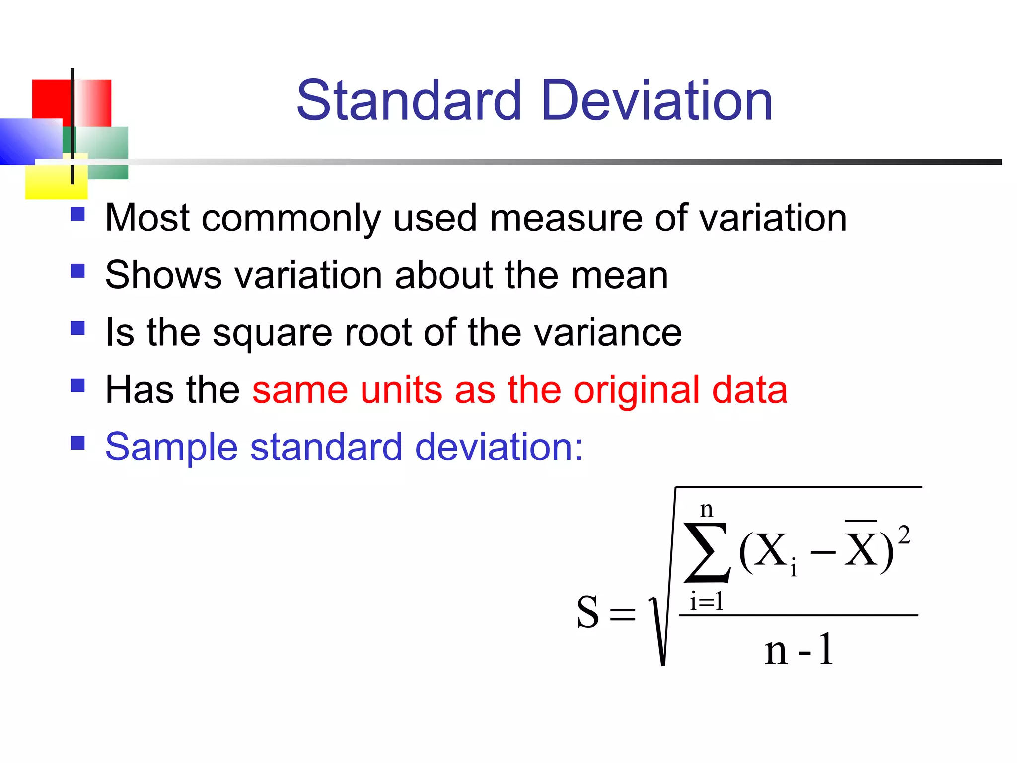
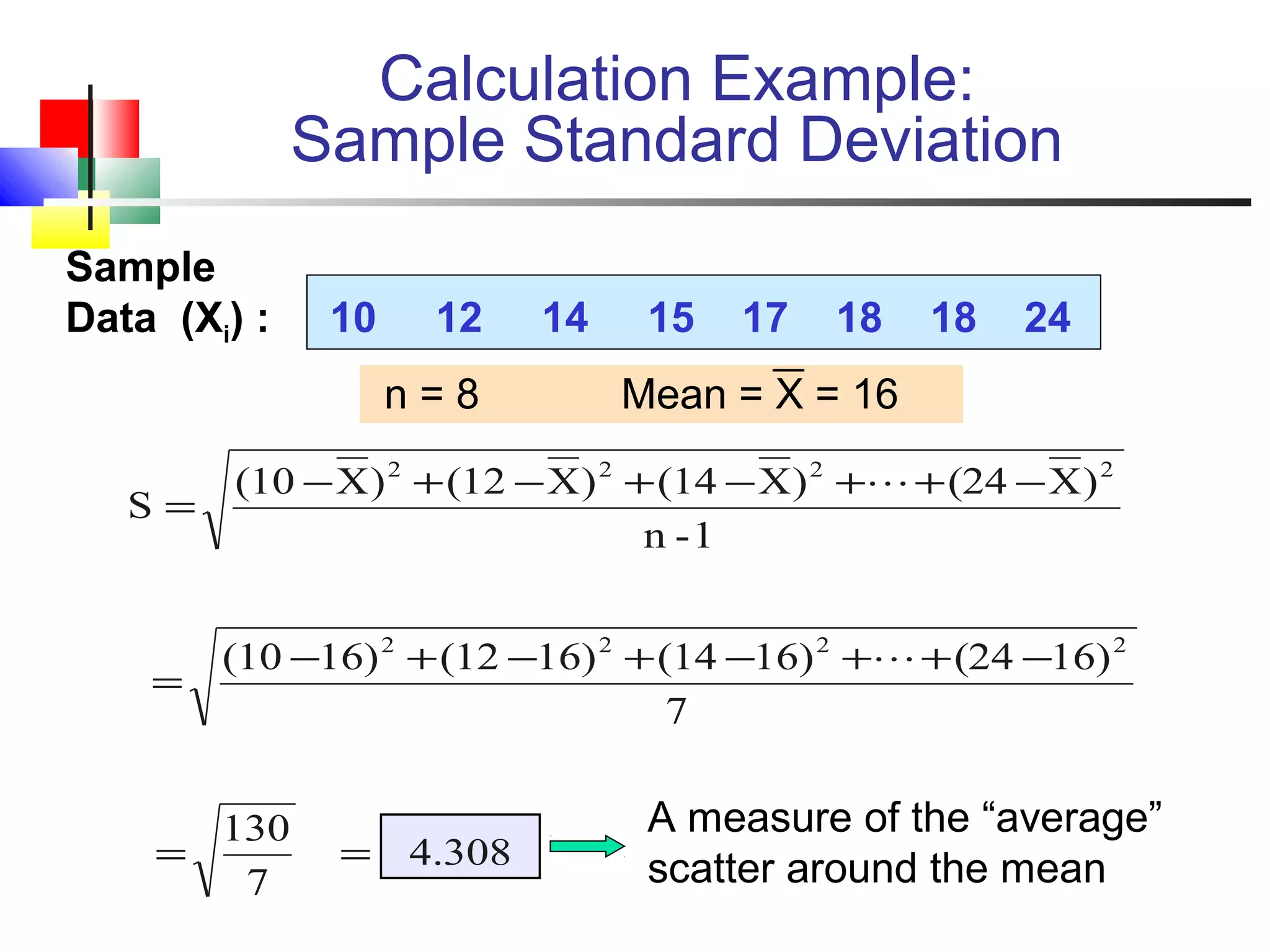
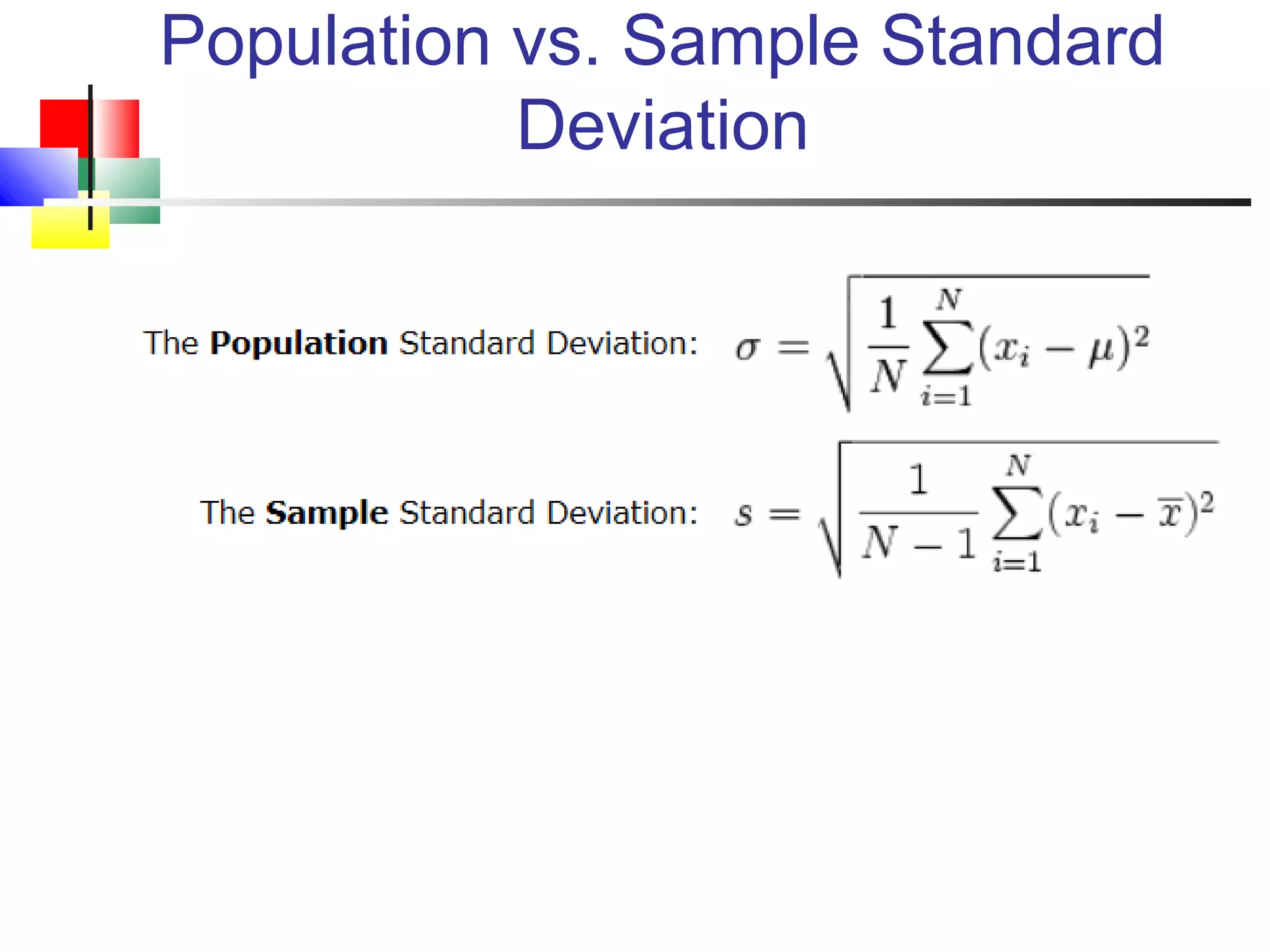
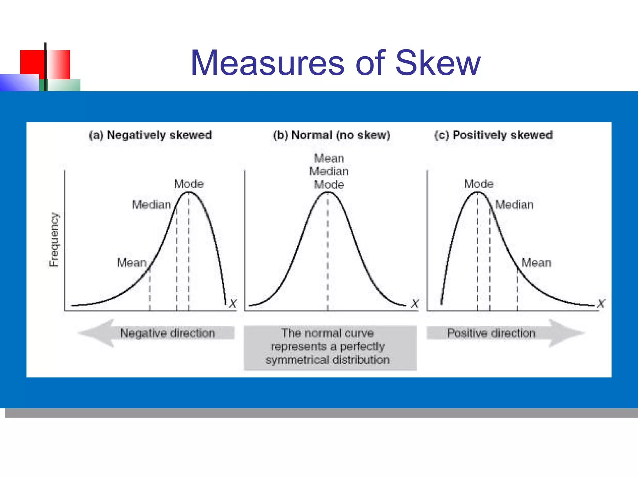
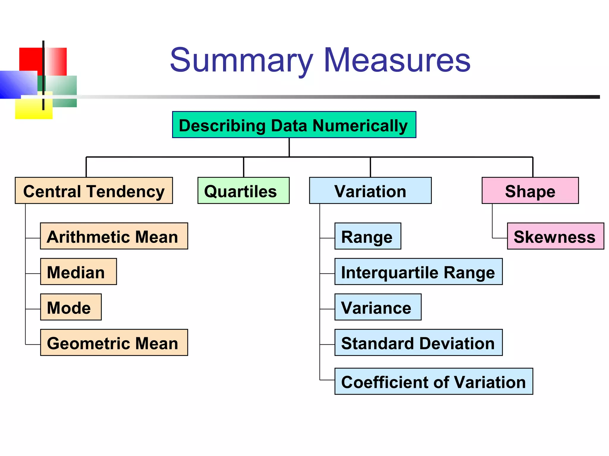
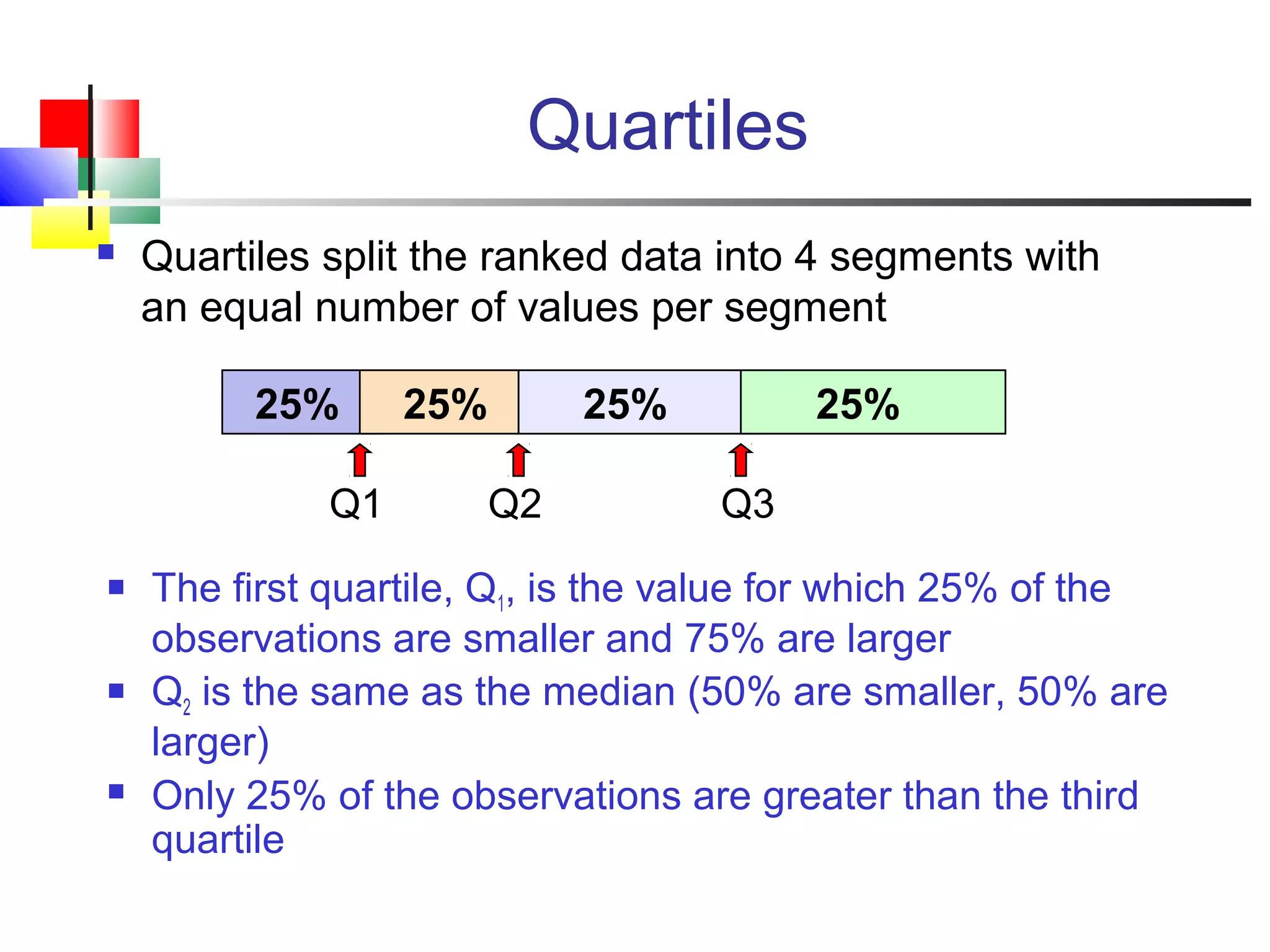
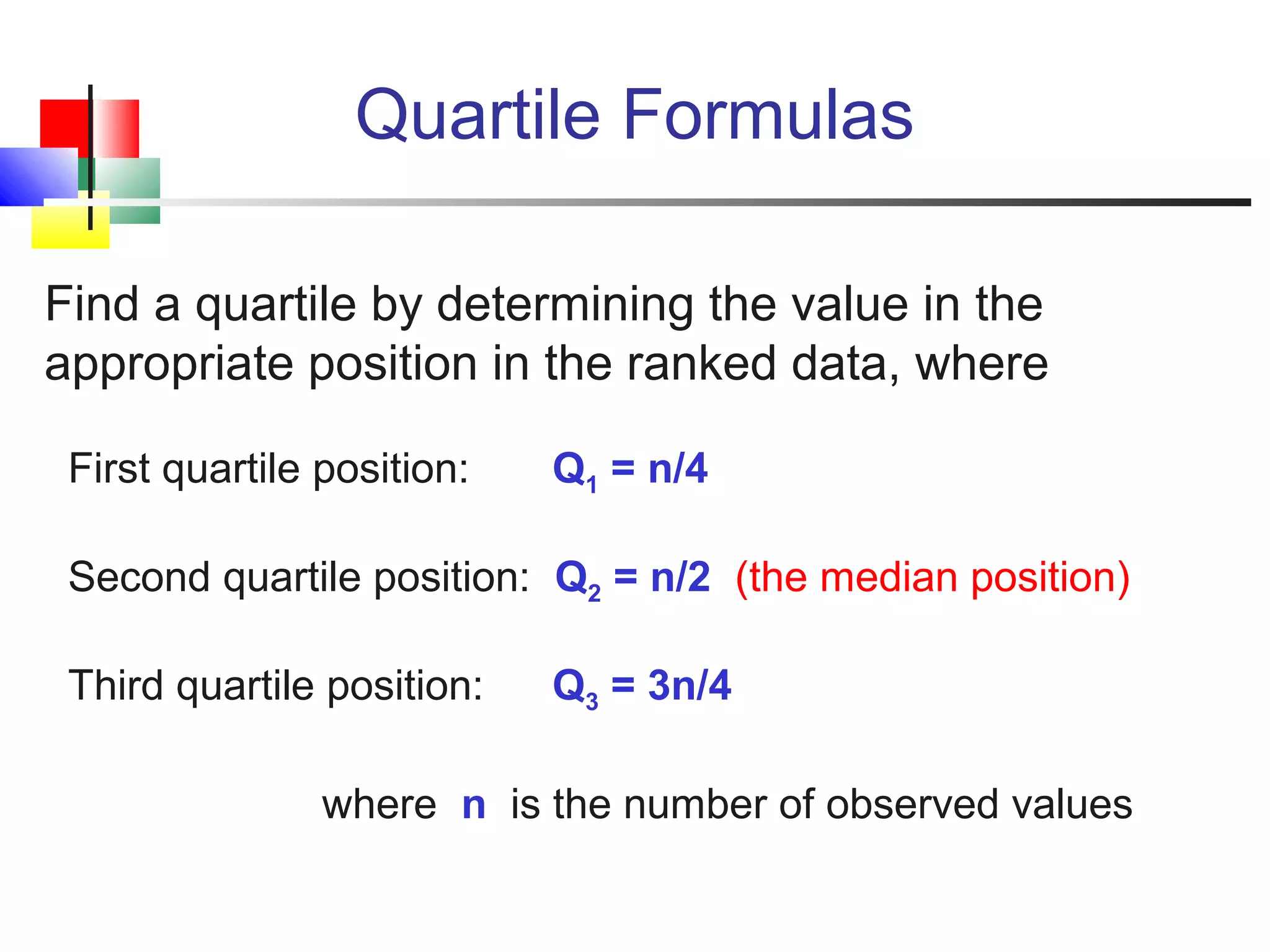
The document discusses various measures of central tendency, dispersion, and shape used to describe data numerically. It defines terms like mean, median, mode, variance, standard deviation, coefficient of variation, range, interquartile range, skewness, and quartiles. It provides formulas and examples of how to calculate these measures from data sets. The document also discusses concepts like normal distribution, empirical rule, and how measures of central tendency and dispersion do not provide information about the shape or symmetry of a distribution.

1. AGBS | Bangalore
Measures of Dispersion

2. Summary Measures
Arithmetic Mean
Median
Mode
Describing Data Numerically
Variance
Standard Deviation
Coefficient of Variation
Range
Interquartile Range
Geometric Mean
Skewness
Central Tendency Variation ShapeQuartiles

3. Quartiles
 Quartiles split the ranked data into 4 segments with
an equal number of values per segment
25% 25% 25% 25%
 The first quartile, Q1, is the value for which 25% of the
observations are smaller and 75% are larger
 Q2 is the same as the median (50% are smaller, 50% are
larger)
 Only 25% of the observations are greater than the third
quartile
Q1 Q2 Q3

4. Quartile Formulas
Find a quartile by determining the value in the
appropriate position in the ranked data, where
First quartile position: Q1 = n/4
Second quartile position: Q2 = n/2 (the median position)
Third quartile position: Q3 = 3n/4
where n is the number of observed values

5. (n = 9)
Q1 is in the 9/4 = 2.25 position of the ranked data
so Q1 = 12.25
Quartiles
Sample Data in Ordered Array: 11 12 13 16 16 17 18 21 22
 Example: Find the first quartile
Q1 and Q3 are measures of noncentral location
Q2 = median, a measure of central tendency

6. Quartiles
 Example:
(continued)
Overtime
Hours
10-15 15-20 20-25 25-30 30-35 35-40 Total
No. of
employees
11 20 35 20 8 6 100
Calculate Median, First Quartile, 7th
Decile & Interquartile Range

7. Same center,
different variation
Measures of Variation
Variation
Variance Standard
Deviation
Coefficient
of Variation
Range Interquartile
Range
 Measures of variation give
information on the spread or
variability of the data
values.

8. Range
 Simplest measure of variation
 Difference between the largest and the smallest
values in a set of data:
Range = Xlargest – Xsmallest
0 1 2 3 4 5 6 7 8 9 10 11 12 13 14
Range = 14 - 1 = 13
Example:

9.  Ignores the way in which data are distributed
 Sensitive to outliers
7 8 9 10 11 12
Range = 12 - 7 = 5
7 8 9 10 11 12
Range = 12 - 7 = 5
Disadvantages of the Range
1,1,1,1,1,1,1,1,1,1,1,2,2,2,2,2,2,2,2,3,3,3,3,4,5
1,1,1,1,1,1,1,1,1,1,1,2,2,2,2,2,2,2,2,3,3,3,3,4,120
Range = 5 - 1 = 4
Range = 120 - 1 = 119

10. Coefficient of Range
Coefficient of Range = [L-S]/[L+S]
Where,
L = Largest value in the data set
S = Smallest value in the data set

11. Interquartile Range
 Can eliminate some outlier problems by using
the interquartile range
 Eliminate some high- and low-valued
observations and calculate the range from the
remaining values
 Interquartile range = 3rd
quartile – 1st
quartile
= Q3 – Q1

12. Interquartile Range
Median
(Q2)
X
maximumX
minimum Q1 Q3
Example:
25% 25% 25% 25%
12 30 45 57 70
Interquartile range
= 57 – 30 = 27

13. Coefficient of QD
Coefficient of QD= [Q3-Q1]/[Q3+Q1]

14. Average Deviation
Coefficient of AD = (Average Deviation)/(Mean or Median)

15. Calculate the Coefficient of AD
(mean)
Sales (in thousand Rs) No. of days
10-20 3
20-30 6
30-40 11
40-50 3
50-60 2

16.  Average (approximately) of squared deviations
of values from the mean
 Sample variance:
Variance
1-n
)X(X
S
n
1i
2
i
2
∑=
−
=
Where = mean
n = sample size
Xi = ith
value of the variable X
X

17. Standard Deviation
 Most commonly used measure of variation
 Shows variation about the mean
 Is the square root of the variance
 Has the same units as the original data
 Sample standard deviation:
1-n
)X(X
S
n
1i
2
i∑=
−
=

18. Calculation Example:
Sample Standard Deviation
Sample
Data (Xi) : 10 12 14 15 17 18 18 24
n = 8 Mean = X = 16
4.308
7
130
7
16)(2416)(1416)(1216)(10
1-n
)X(24)X(14)X(12)X(10
S
2222
2222
==
−++−+−+−
=
−++−+−+−
=


A measure of the “average”
scatter around the mean

19. Population vs. Sample Standard
Deviation

20. Population vs. Sample Standard
Deviation (Grouped Data)

21. Calculate the Standard Deviation
for the following sample
Number of pins knocked down in ten-pin bowling matches

22. Solution
Number of pins knocked down in ten-pin bowling matches

23. Calculate the Standard Deviation
for the following sample
Heights of students

24. Solution

25. Calculate the Standard Deviation
for the following sample
Number of typing errors

26. Comparing Standard Deviations
Mean = 15.5
S = 3.33811 12 13 14 15 16 17 18 19 20 21
11 12 13 14 15 16 17 18 19 20 21
Data B
Data A
Mean = 15.5
S = 0.926
11 12 13 14 15 16 17 18 19 20 21
Mean = 15.5
S = 4.567
Data C

27. Measuring variation
Small standard deviation
Large standard deviation

28. Advantages of Variance and
Standard Deviation
 Each value in the data set is used in the
calculation
 Values far from the mean are given extra
weight
(because deviations from the mean are squared)

29. Coefficient of Variation
 Measures relative variation
 Always in percentage (%)
 Shows variation relative to mean
 Can be used to compare two or more sets of
data measured in different units
100%
X
S
CV ⋅







=

30. Comparing Coefficient
of Variation
 Stock A:
 Average price last year = $50
 Standard deviation = $5
 Stock B:
 Average price last year = $100
 Standard deviation = $5
Both stocks
have the same
standard
deviation, but
stock B is less
variable relative
to its price
10%100%
$50
$5
100%
X
S
CVA =⋅=⋅







=
5%100%
$100
$5
100%
X
S
CVB =⋅=⋅







=

31. Sample vs. Population CV

32. Calculate!
 Calculate the coefficient of variation for
the following data set.
 The price, in cents, of a stock over five trading days
was 52, 58, 55, 57, 59.

33. Solution

34. Pooled Standard Deviation

35. Pooled Standard Deviation

36. Z Scores
 A measure of distance from the mean (for example, a
Z-score of 2.0 means that a value is 2.0 standard
deviations from the mean)
 The difference between a value and the mean, divided
by the standard deviation
 A Z score above 3.0 or below -3.0 is considered an
outlier
S
XX
Z
−
=

37. Z Scores
Example:
 If the mean is 14.0 and the standard deviation is 3.0,
what is the Z score for the value 18.5?
 The value 18.5 is 1.5 standard deviations above the
mean
 (A negative Z-score would mean that a value is less
than the mean)
1.5
3.0
14.018.5
S
XX
Z =
−
=
−
=
(continued)

38. Shape of a Distribution
 Describes how data are distributed
 Measures of shape
 Symmetric or skewed
Mean = MedianMean < Median Median < Mean
Right-SkewedLeft-Skewed Symmetric

39.  If the data distribution is approximately
bell-shaped, then the interval:
 contains about 68% of the values in
the population or the sample
The Empirical Rule
1σμ ±
μ
68%
1σμ ±

40.  contains about 95% of the values in
the population or the sample
 contains about 99.7% of the values
in the population or the sample
The Empirical Rule
2σμ ±
3σμ ±
3σμ ±
99.7%95%
2σμ ±

42.  Regardless of how the data are distributed,
at least (1 - 1/k2
) x 100% of the values will
fall within k standard deviations of the mean
(for k > 1)
 Examples:
(1 - 1/12
) x 100% = 0% ……..... k=1 (μ ± 1σ)
(1 - 1/22
) x 100% = 75% …........ k=2 (μ ± 2σ)
(1 - 1/32
) x 100% = 89% ………. k=3 (μ ± 3σ)
Chebyshev Rule
withinAt least

43. Calculate!
 Calculate the mean & the standard dev.
 Calculate the percentage of
observations between the mean & 2σ±
Variable Frequency
44-46 3
46-48 24
48-50 27
50-52 21
52-54 5

44. Find the correct Mean & Std. dev.
The Mean & Standard Deviation of a set of 100
observations were worked out as 40 & 5
respectively. It was later learnt that a mistake had
been made in data entry – in place of 40 (the
correct value), 50 was entered.

45. Skewness
 A fundamental task in many statistical analyses is to
characterize the location and variability of a data set
(Measures of central tendency vs. measures of
dispersion)
 Both measures tell us nothing about the shape of the
distribution
 It is possible to have frequency distributions which differ
widely in their nature and composition and yet may
have same central tendency and dispersion.
 Therefore, a further characterization of the data
includes skewness

46. Positive & Negative Skew
 Positive skewness
 There are more observations below the mean than
above it
 When the mean is greater than the median
 Negative skewness
 There are a small number of low observations and a
large number of high ones
 When the median is greater than the mean

47. Measures of Skew
 Skew is a measure of symmetry in the
distribution of scores
Positive
Skew
Negative Skew
Normal
(skew = 0)

48. Measures of Skew

49. The Rules
I. Rule One. If the mean is less than the median,
the data are skewed to the left.
II. Rule Two. If the mean is greater than the
median, the data are skewed to the right.

50. Karl Pearson Coefficient of Skewness

51. Karl Pearson Coefficient - Properties
Advantage – Uses the data completely
Disadvantage – Is sensitive to extreme values

52. Calculate!
 Calculate the coefficient of skewness & comment on
its value

53. Calculate!
 Calculate the coefficient of skewness & comment on
its value
Profits (lakhs) No. of Companies
100-120 17
120-140 53
140-160 199
160-180 194
180-200 327
200-220 208
220-240 2

54. Bowley’s Coefficient of Skewness

55. Bowley’s Coefficient - Properties
Advantage – Is not sensitive to extreme values
Disadvantage – Does not use the data completely

56. Calculate!

57. Kelly’s Coefficient of Skewness

58. Calculate!
 Obtain the limits of daily wages of the central 50% of the
workers
 Calculate Bowley’s & Kelly’s Coefficients of Skewness
Wages No. of Workers
Below 200 10
200-250 25
250-300 145
300-350 220
350-400 70
Above 400 30

59. Moments about the Mean