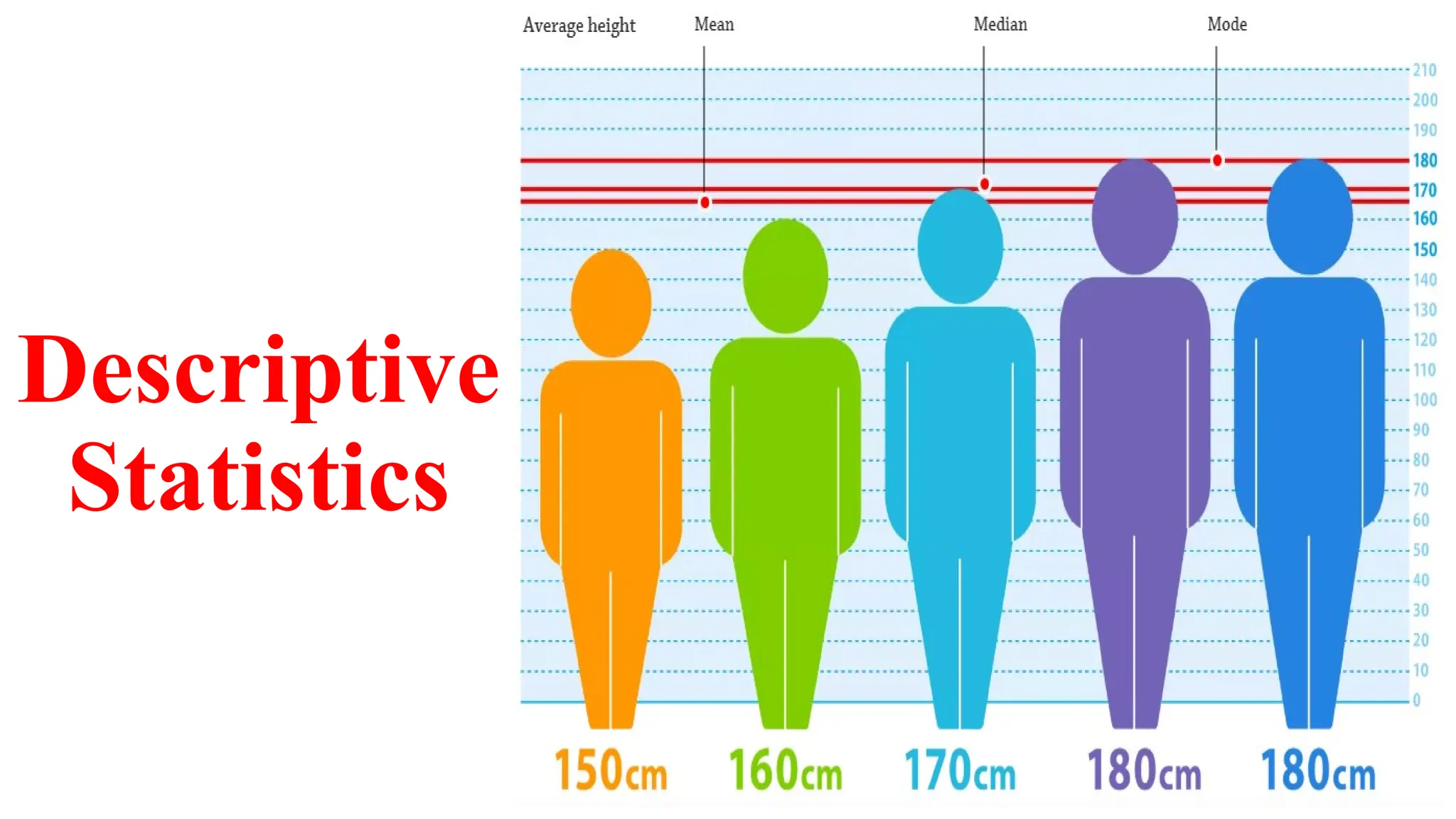
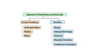
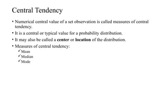
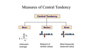
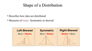
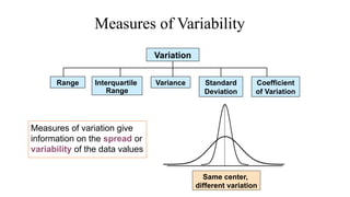
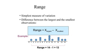
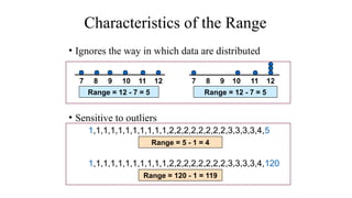
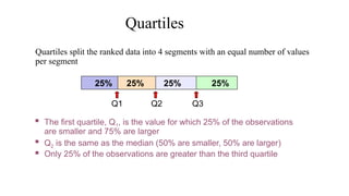
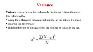
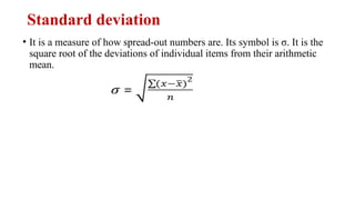
The document describes various statistical measures, focusing on measures of central tendency (mean, median, and mode) and their properties, advantages, and limitations. It also explains dispersion measures like range, variance, standard deviation, and coefficient of variation, highlighting their significance in understanding data variability. Additionally, it introduces percentiles and standard error as tools for analyzing and interpreting statistical data.

![Examples
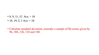
Calculate standard deviation, consider a sample of IQ scores given by 96,
104, 126, 134 and 140.
The mean of this data is (96+104+126+134+140)/5 =120.
σ = √[ ∑(x-120)^2 / 5 ]
The deviation from the mean is given by
96-120 = -24,
104-120 = -16,
126-120 = 6,
134-120 = 14,
140-120 = 20.
σ = √[ ((-24)^2+(-16)^2+(6)^2+(14)^2+(20)^2) / 5 ]
σ = √[ (1464) / 5 ] = ± 17.11](https://image.slidesharecdn.com/descriptivestatistics-241006083431-4722ffcb/85/Descriptive-statistics-Mean-Mode-Median-36-320.jpg)