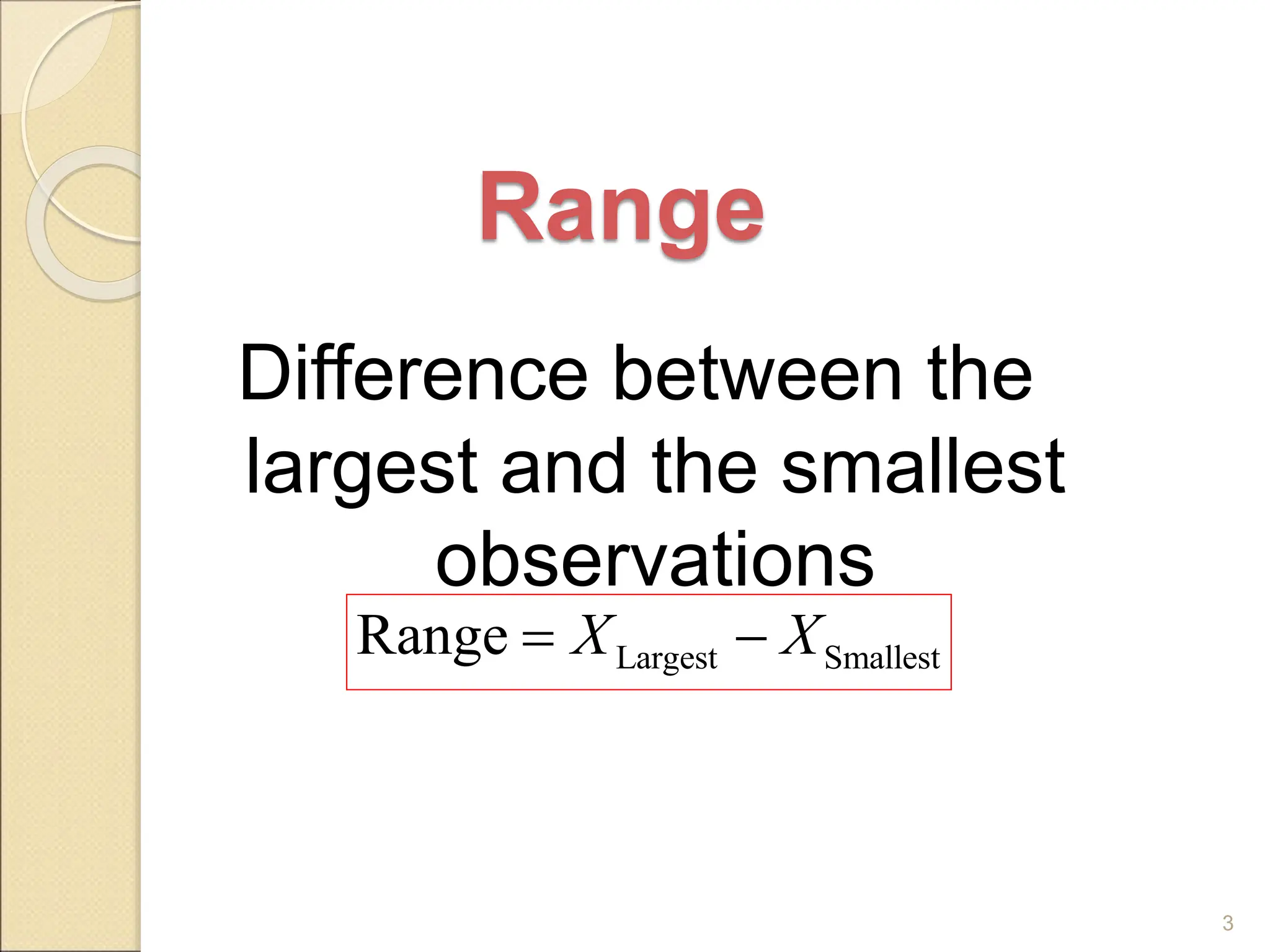
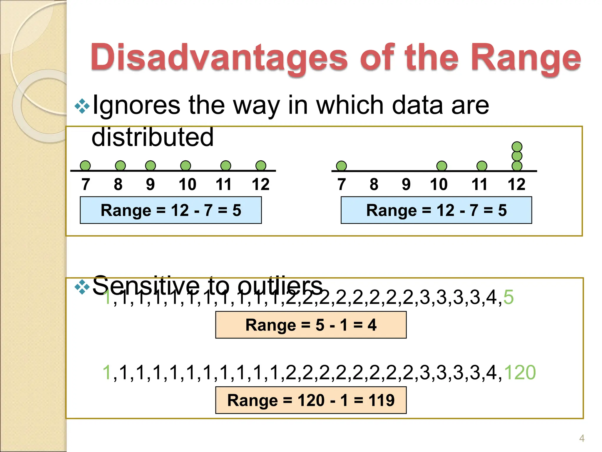
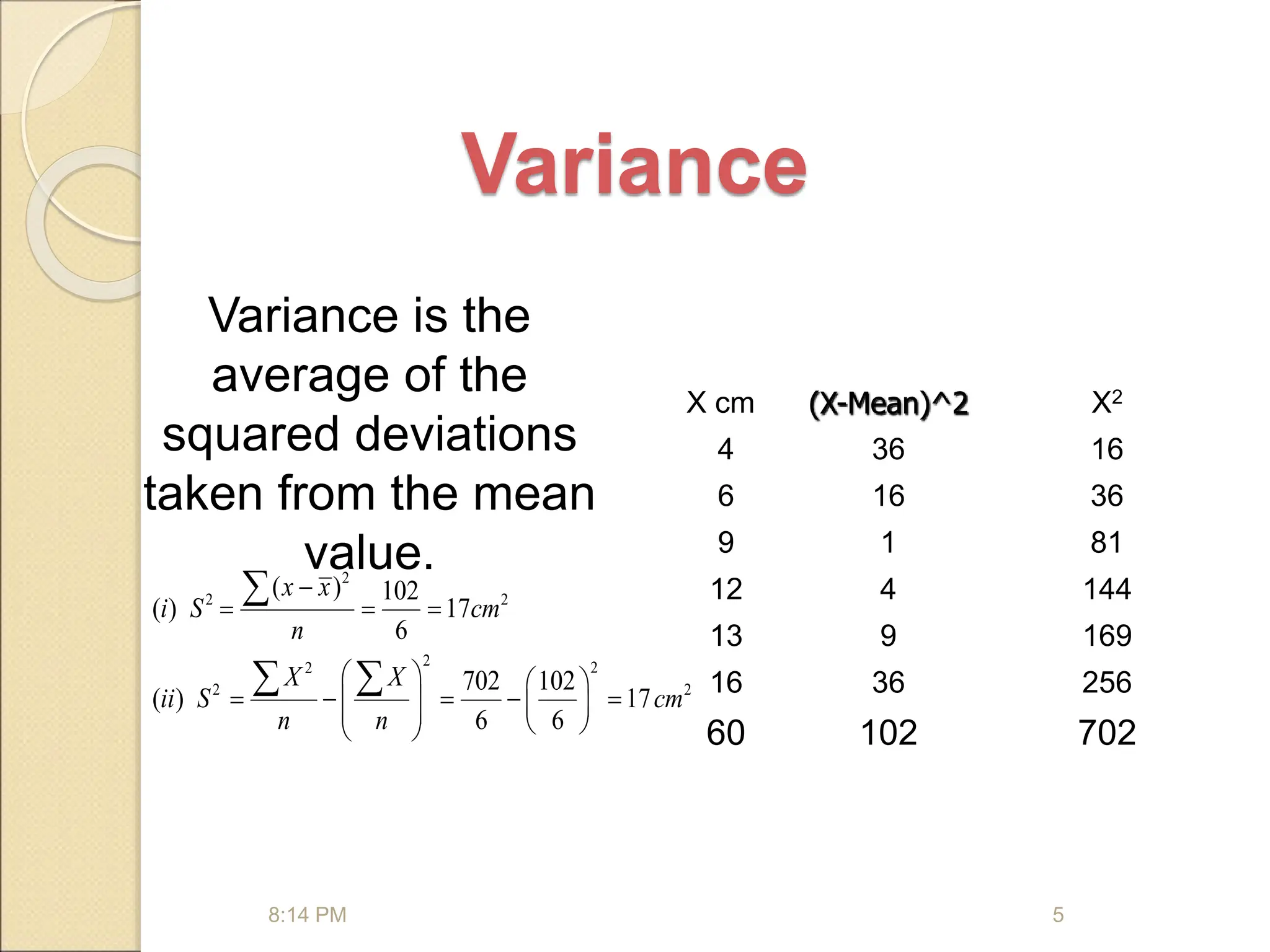
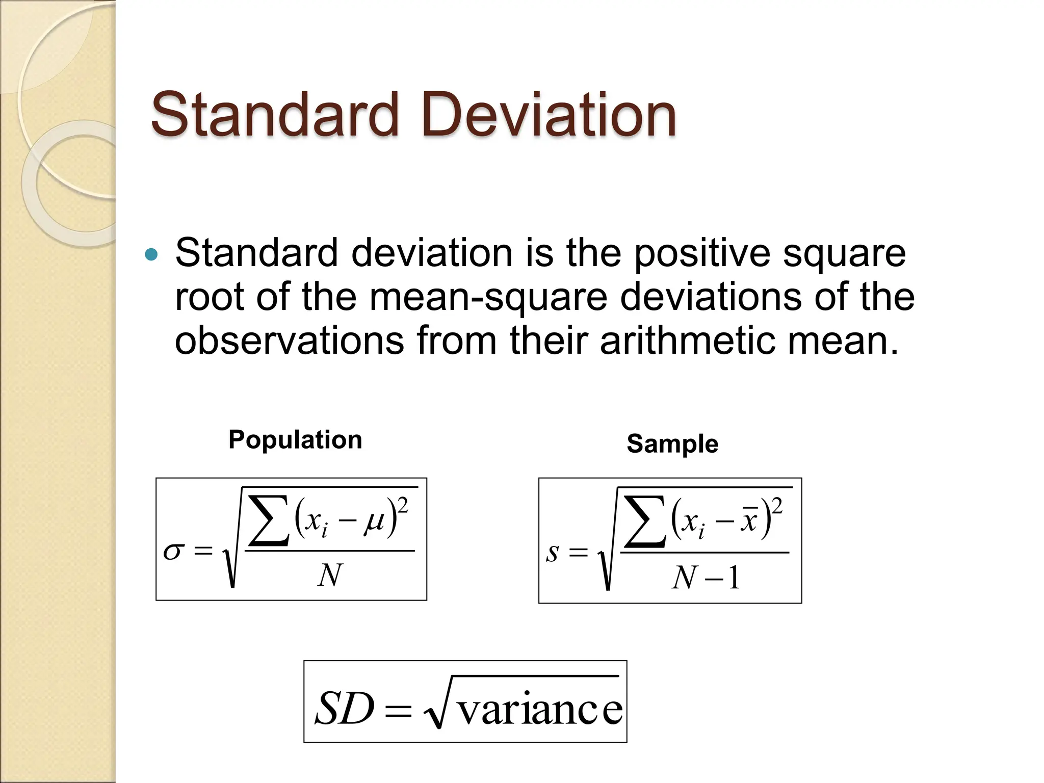
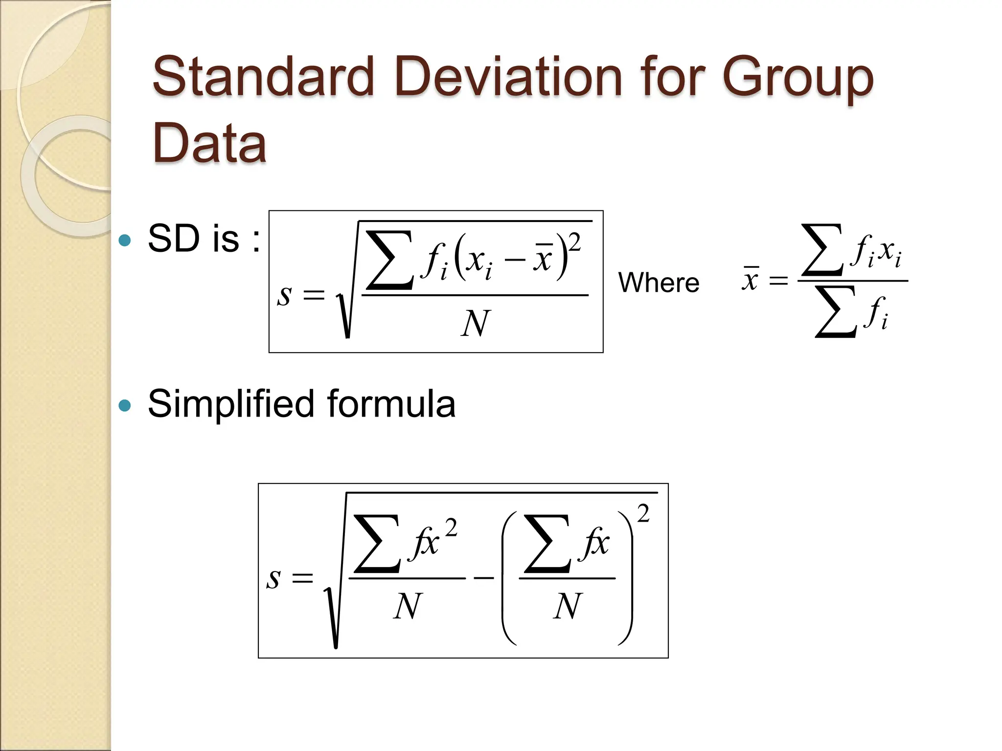
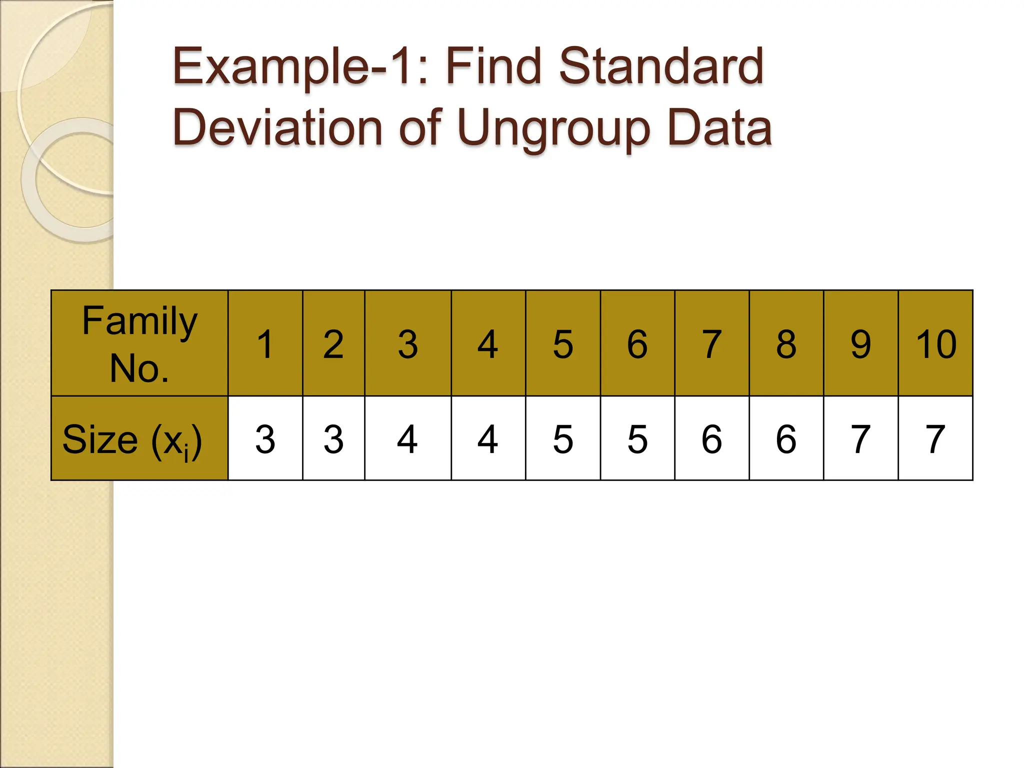
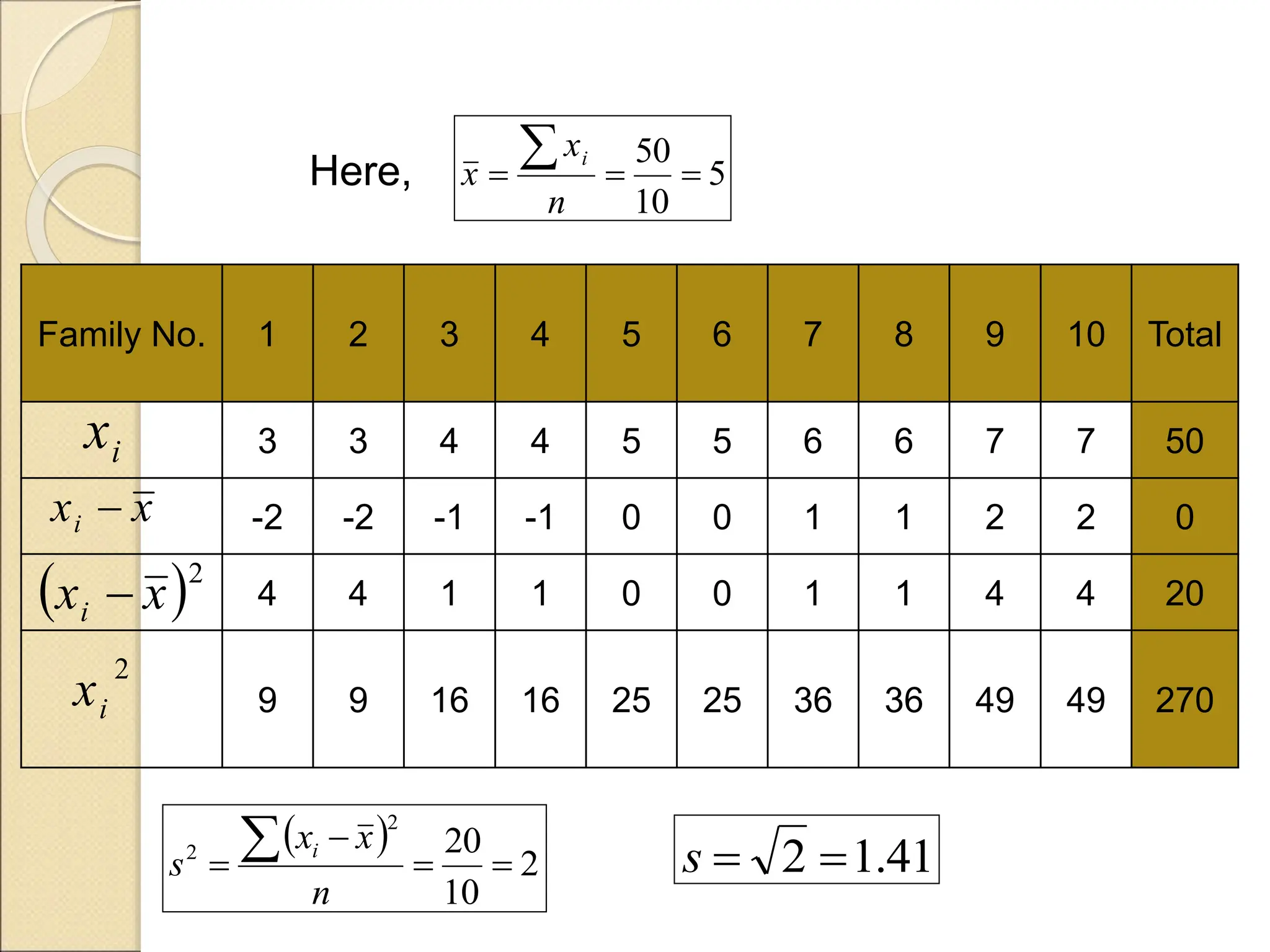
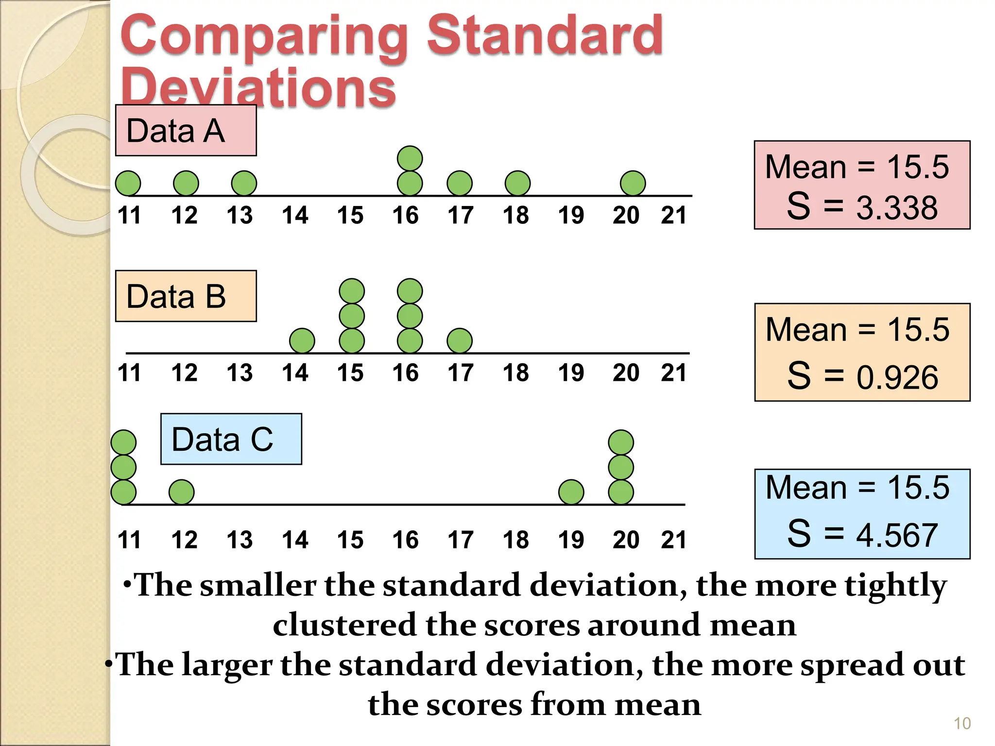
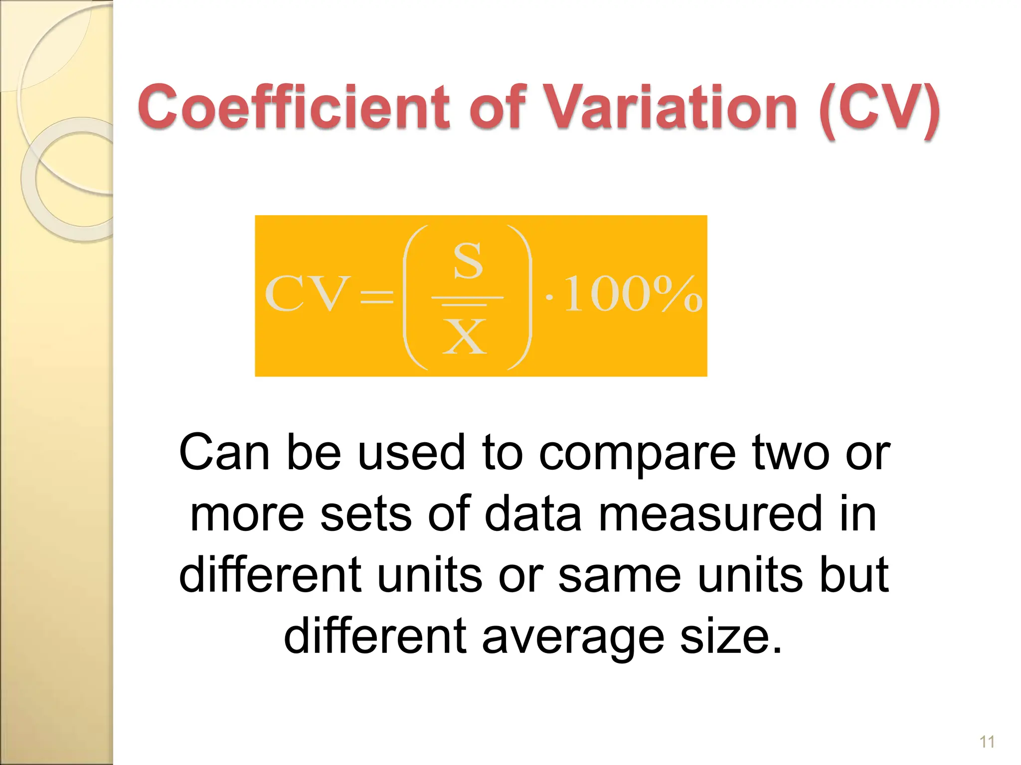
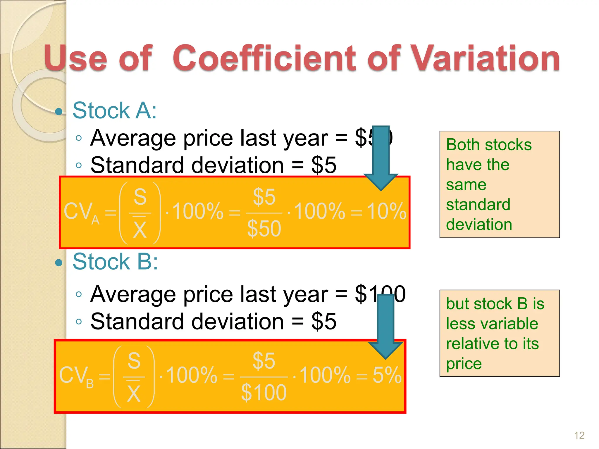
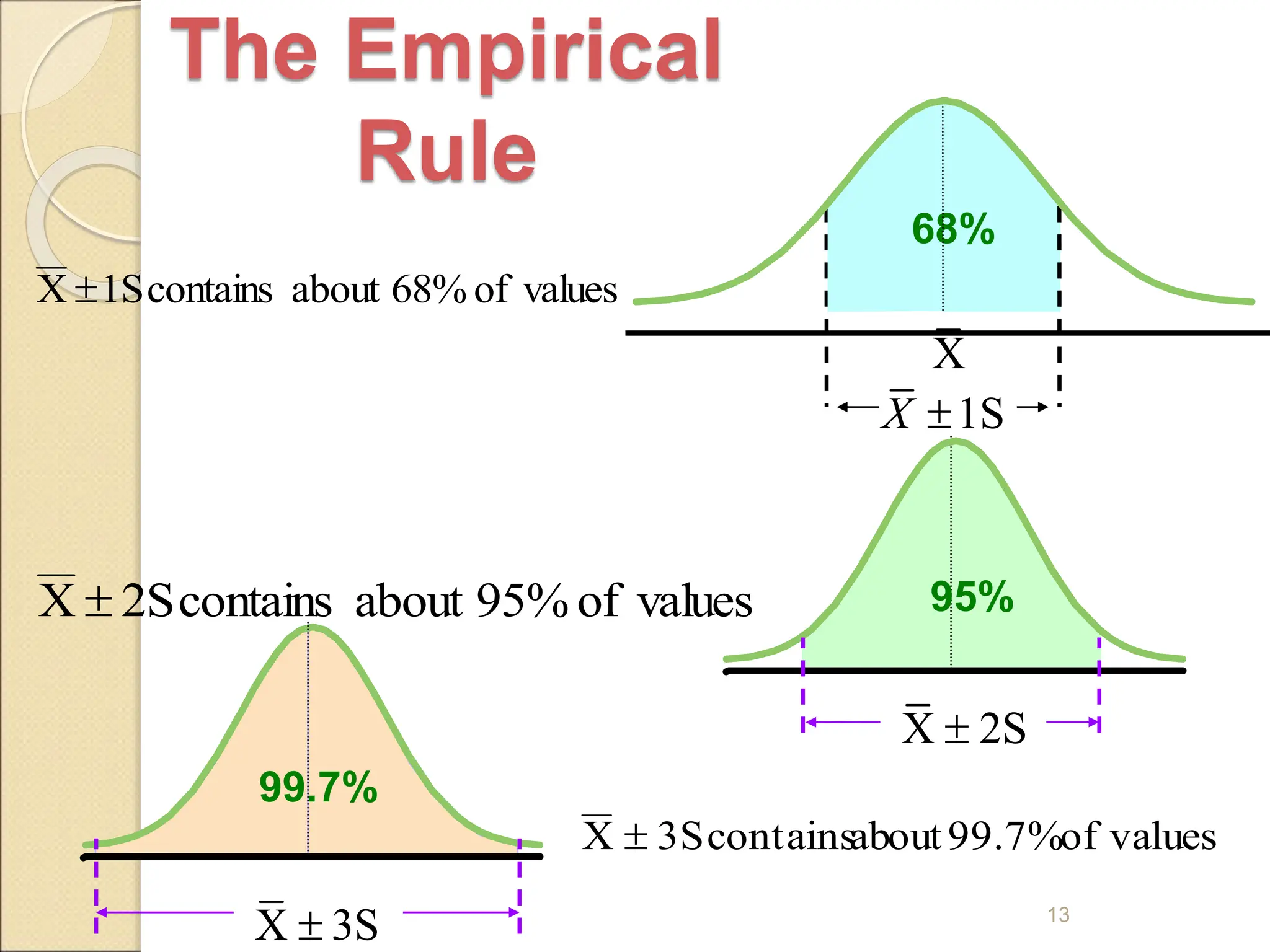
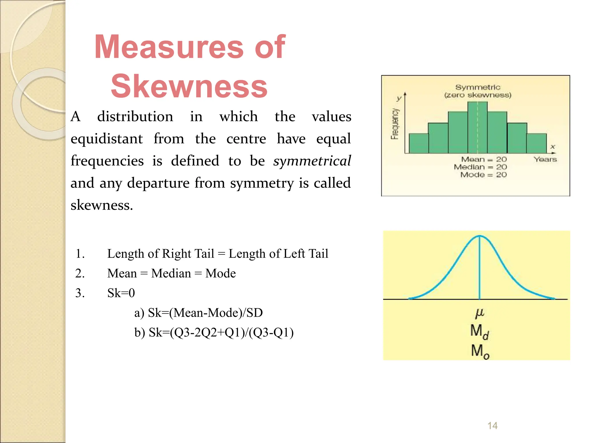
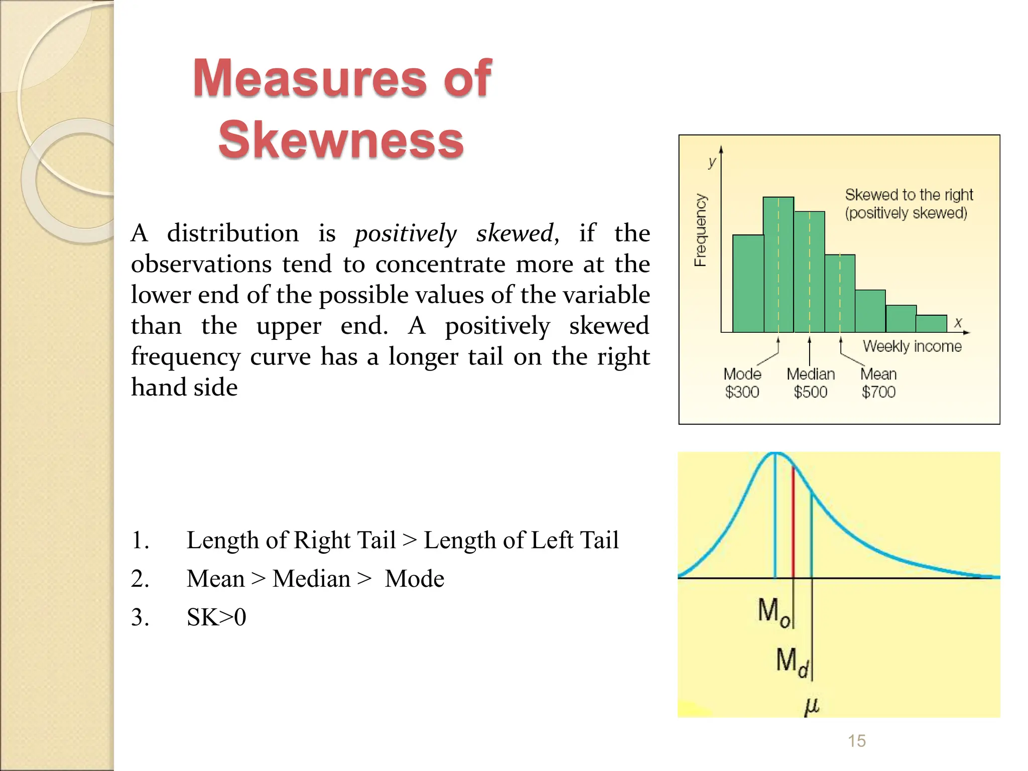
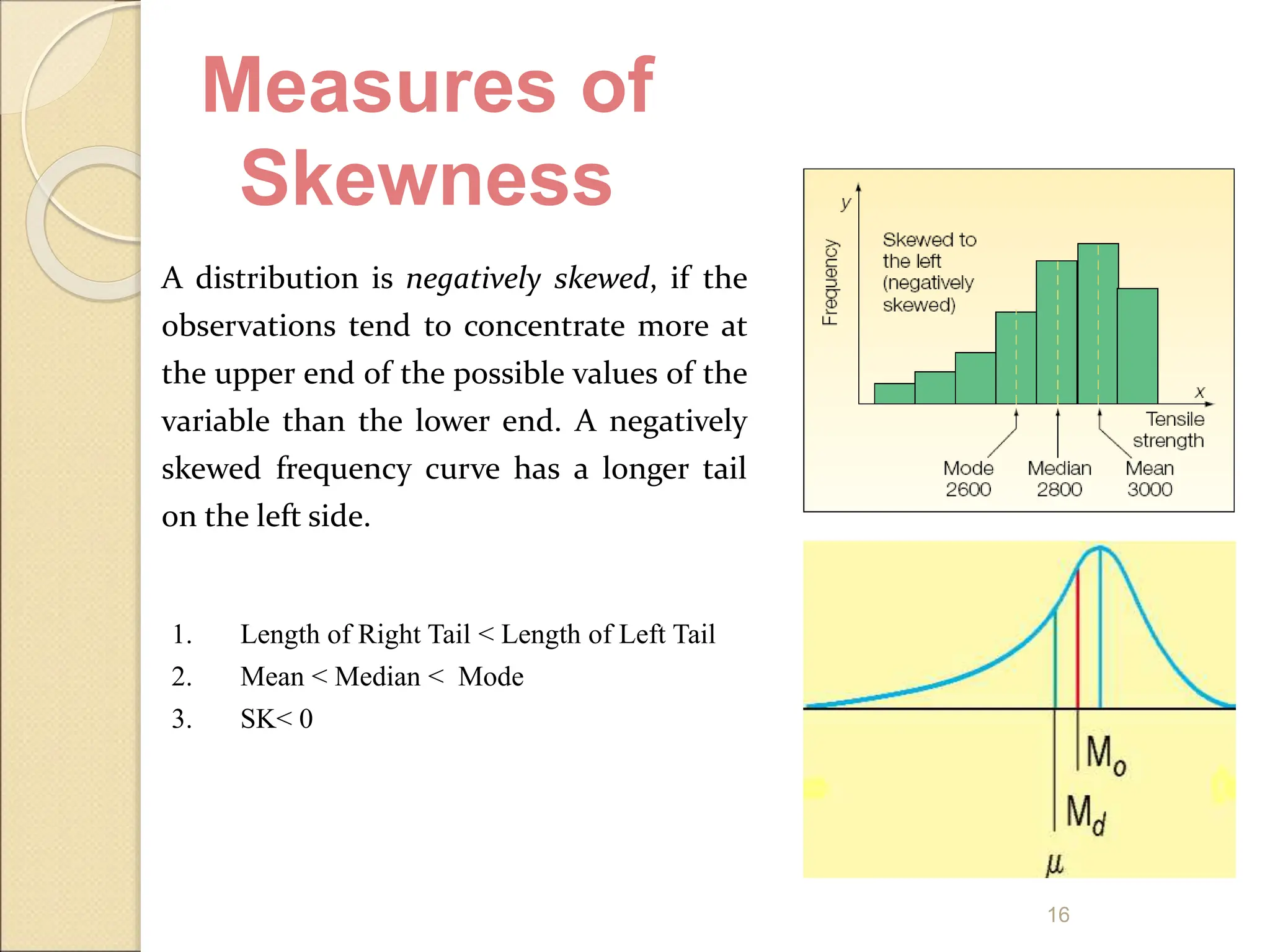
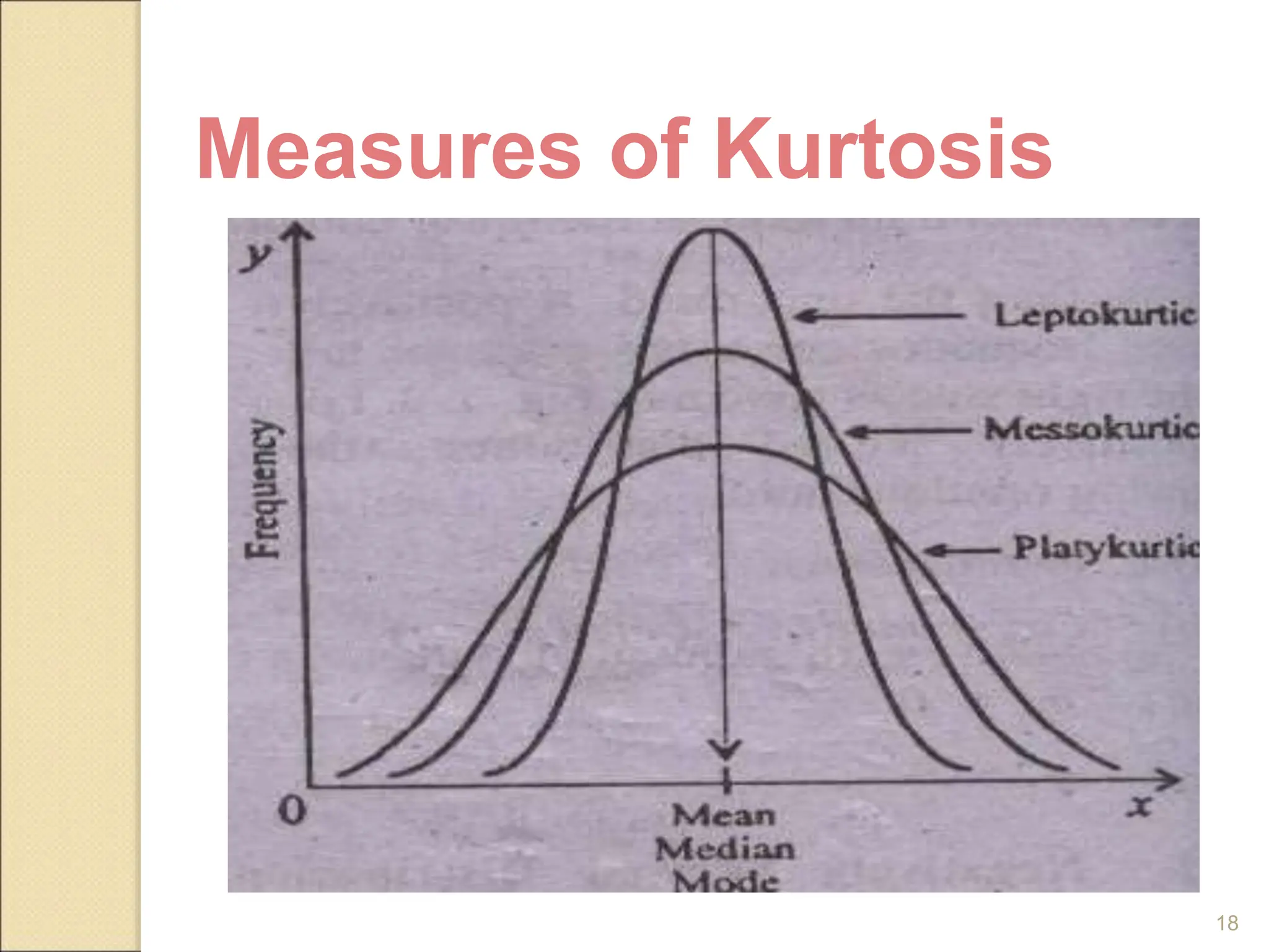
Measures of dispersion quantify the spread of values in a dataset, including range, variance, and standard deviation. The range indicates the difference between the highest and lowest values, while variance and standard deviation assess the average squared deviation from the mean. The coefficient of variation allows comparisons across different data sets, and skewness and kurtosis provide insights into the shape of the distribution.

1. Measures of Dispersion
Measures of variation measure
the variation present among the
values of a data set, so measures
of variation are measures of
spread of values in the data.
1

2. 2
Absolute Measures of
Dispersion
Range
Quartile Deviation
Mean Deviation
Variance and Standard Deviation

3. Range
Difference between the
largest and the smallest
observations
3
Largest Smallest
Range X X
 

4. Disadvantages of the Range
Ignores the way in which data are
distributed
Sensitive to outliers
4
7 8 9 10 11 12
Range = 12 - 7 = 5
7 8 9 10 11 12
Range = 12 - 7 = 5
1,1,1,1,1,1,1,1,1,1,1,2,2,2,2,2,2,2,2,3,3,3,3,4,5
1,1,1,1,1,1,1,1,1,1,1,2,2,2,2,2,2,2,2,3,3,3,3,4,120
Range = 5 - 1 = 4
Range = 120 - 1 = 119

5. Variance
Variance is the
average of the
squared deviations
taken from the mean
value.
2
2 2
2 2
2
2 2
( ) 102
( ) 17
6
702 102
( ) 17
6 6
x x
i S cm
n
X X
ii S cm
n n

  
   
    
   
   
 

 
8:14 PM 5
X cm (X-Mean)^2 X2
4 36 16
6 16 36
9 1 81
12 4 144
13 9 169
16 36 256
60 102 702

6. Standard Deviation
 Standard deviation is the positive square
root of the mean-square deviations of the
observations from their arithmetic mean.
variance

SD
 
1
2




N
x
x
s
i
 
N
xi
 

2


Population Sample

7. Standard Deviation for Group
Data
 SD is :
 Simplified formula
2
2












N
fx
N
fx
s
 
N
x
x
f
s
i
i
 

2



i
i
i
f
x
f
x
Where

8. Example-1: Find Standard
Deviation of Ungroup Data
Family
No.
1 2 3 4 5 6 7 8 9 10
Size (xi) 3 3 4 4 5 5 6 6 7 7

9. i
x
x
xi 
 2
x
xi 
2
i
x
Family No. 1 2 3 4 5 6 7 8 9 10 Total
3 3 4 4 5 5 6 6 7 7 50
-2 -2 -1 -1 0 0 1 1 2 2 0
4 4 1 1 0 0 1 1 4 4 20
9 9 16 16 25 25 36 36 49 49 270
5
10
50




n
x
x
i
 
2
10
20
2
2





n
x
x
s i
41
.
1
2 

s
Here,

10. Comparing Standard
Deviations
10
Mean = 15.5
S = 3.338
11 12 13 14 15 16 17 18 19 20 21
Data A
11 12 13 14 15 16 17 18 19 20 21
Mean = 15.5
S = 4.567
Data C
•The smaller the standard deviation, the more tightly
clustered the scores around mean
•The larger the standard deviation, the more spread out
the scores from mean
11 12 13 14 15 16 17 18 19 20 21
Data B
Mean = 15.5
S = 0.926

11. Coefficient of Variation (CV)
Can be used to compare two or
more sets of data measured in
different units or same units but
different average size.
11
100%
X
S
CV 










12. Use of Coefficient of Variation
 Stock A:
◦ Average price last year = $50
◦ Standard deviation = $5
 Stock B:
◦ Average price last year = $100
◦ Standard deviation = $5
12
but stock B is
less variable
relative to its
price
10%
100%
$50
$5
100%
X
S
CVA 












5%
100%
$100
$5
100%
X
S
CVB 












Both stocks
have the
same
standard
deviation

13. values
of
68%
about
contains
1S
X 
values
of
99.7%
about
contains
3S
X 
13
The Empirical
Rule
X
68%
1S
X 
values
of
95%
about
contains
2S
X  95%
X 2S

X 3S

99.7%

14. 14
A distribution in which the values
equidistant from the centre have equal
frequencies is defined to be symmetrical
and any departure from symmetry is called
skewness.
1. Length of Right Tail = Length of Left Tail
2. Mean = Median = Mode
3. Sk=0
a) Sk=(Mean-Mode)/SD
b) Sk=(Q3-2Q2+Q1)/(Q3-Q1)
Measures of
Skewness

15. 15
A distribution is positively skewed, if the
observations tend to concentrate more at the
lower end of the possible values of the variable
than the upper end. A positively skewed
frequency curve has a longer tail on the right
hand side
1. Length of Right Tail > Length of Left Tail
2. Mean > Median > Mode
3. SK>0
Measures of
Skewness

16. 16
A distribution is negatively skewed, if the
observations tend to concentrate more at
the upper end of the possible values of the
variable than the lower end. A negatively
skewed frequency curve has a longer tail
on the left side.
1. Length of Right Tail < Length of Left Tail
2. Mean < Median < Mode
3. SK< 0
Measures of
Skewness

17. 17
The Kurtosis is the degree of peakedness or flatness of a
unimodal (single humped) distribution,
• When the values of a variable are highly concentrated
around the mode, the peak of the curve becomes relatively
high; the curve is Leptokurtic.
• When the values of a variable have low concentration
around the mode, the peak of the curve becomes relatively
flat;curve is Platykurtic.
• A curve, which is neither very peaked nor very flat-toped,
it is taken as a basis for comparison, is called
Mesokurtic/Normal.
Measures of Kurtosis

18. 18
Measures of Kurtosis