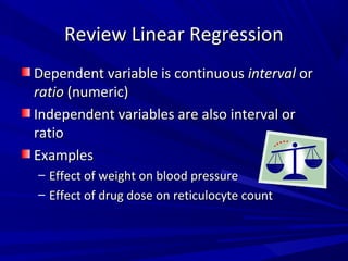
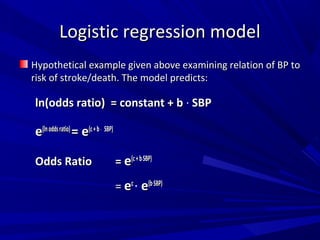
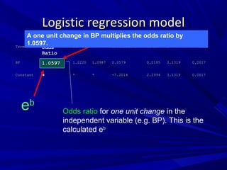
The document discusses logistic regression, highlighting its use for modeling the relationship between continuous independent variables and a binary dependent variable. It explains concepts like odds, log odds ratio, and provides examples of how changes in independent variables affect odds ratios. Statistical significance, coefficients, and their interpretations in practical studies are also addressed.


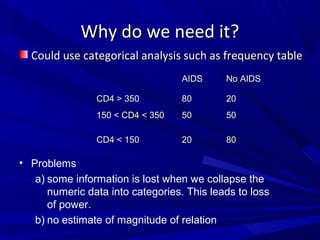


![Relation between probability p and logit
0.000
0.250
0.500
0.750
1.000
-8 -6 -4 -2 0 2 4 6 8
logit = ln[p/(1-p)]](https://image.slidesharecdn.com/logisticregressionblyth2006simplified-131012045023-phpapp02/85/Logistic-regression-blyth-2006-simplified-10-320.jpg)
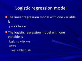


![Dichotomous (yes-no) variablesDichotomous (yes-no) variables
Gender is coded as 0 for male, 1 for femaleGender is coded as 0 for male, 1 for female
eebb
[e[e1.51.5
= 4.48] is change in OR for 1 unit change in gender,= 4.48] is change in OR for 1 unit change in gender,
i.e. OR for females relative to malesi.e. OR for females relative to males
eebb
for any dummy variable (coded 0-1) is the adjustedfor any dummy variable (coded 0-1) is the adjusted
OR for that risk factor, since “1 unit of change” =OR for that risk factor, since “1 unit of change” =
presence vs. absence of risk factorpresence vs. absence of risk factor
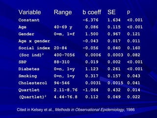
VariableVariable RangeRange b coeffb coeff SESE pp
ConstantConstant -6.376-6.376 1.6341.634 <0.001<0.001
AgeAge 40-69 y40-69 y 0.0860.086 0.1150.115 <0.001<0.001
GenderGender 0=m, 1=f0=m, 1=f 1.5001.500 0.9670.967 0.1210.121](https://image.slidesharecdn.com/logisticregressionblyth2006simplified-131012045023-phpapp02/85/Logistic-regression-blyth-2006-simplified-29-320.jpg)


![logistic model final_pptx__corected_one[1].pptx](https://cdn.slidesharecdn.com/ss_thumbnails/finalpptxcorectedone1-251124022241-c29356b7-thumbnail.jpg?width=640&height=640&fit=bounds)