The document discusses binary logistic regression. Some key points:
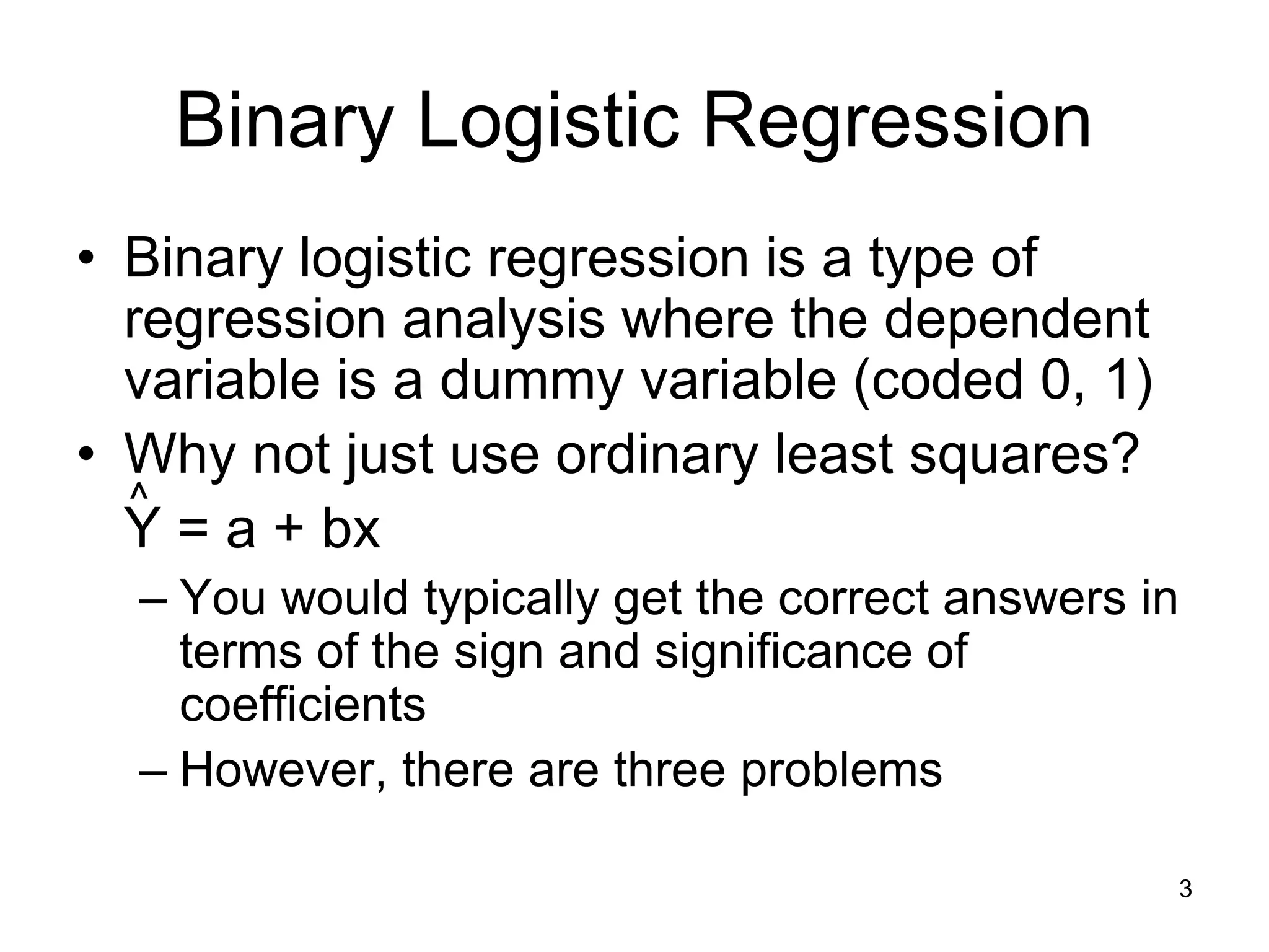
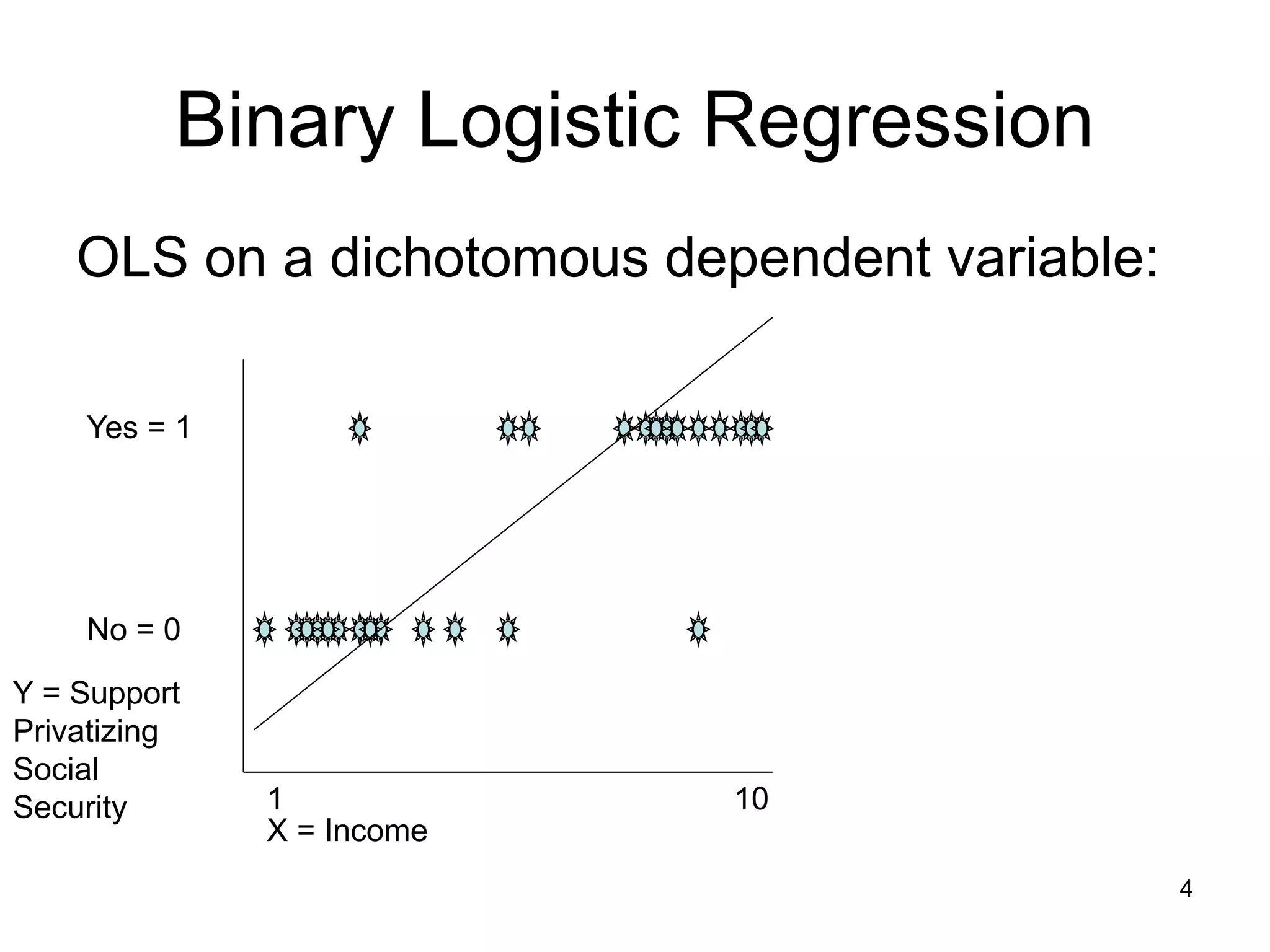
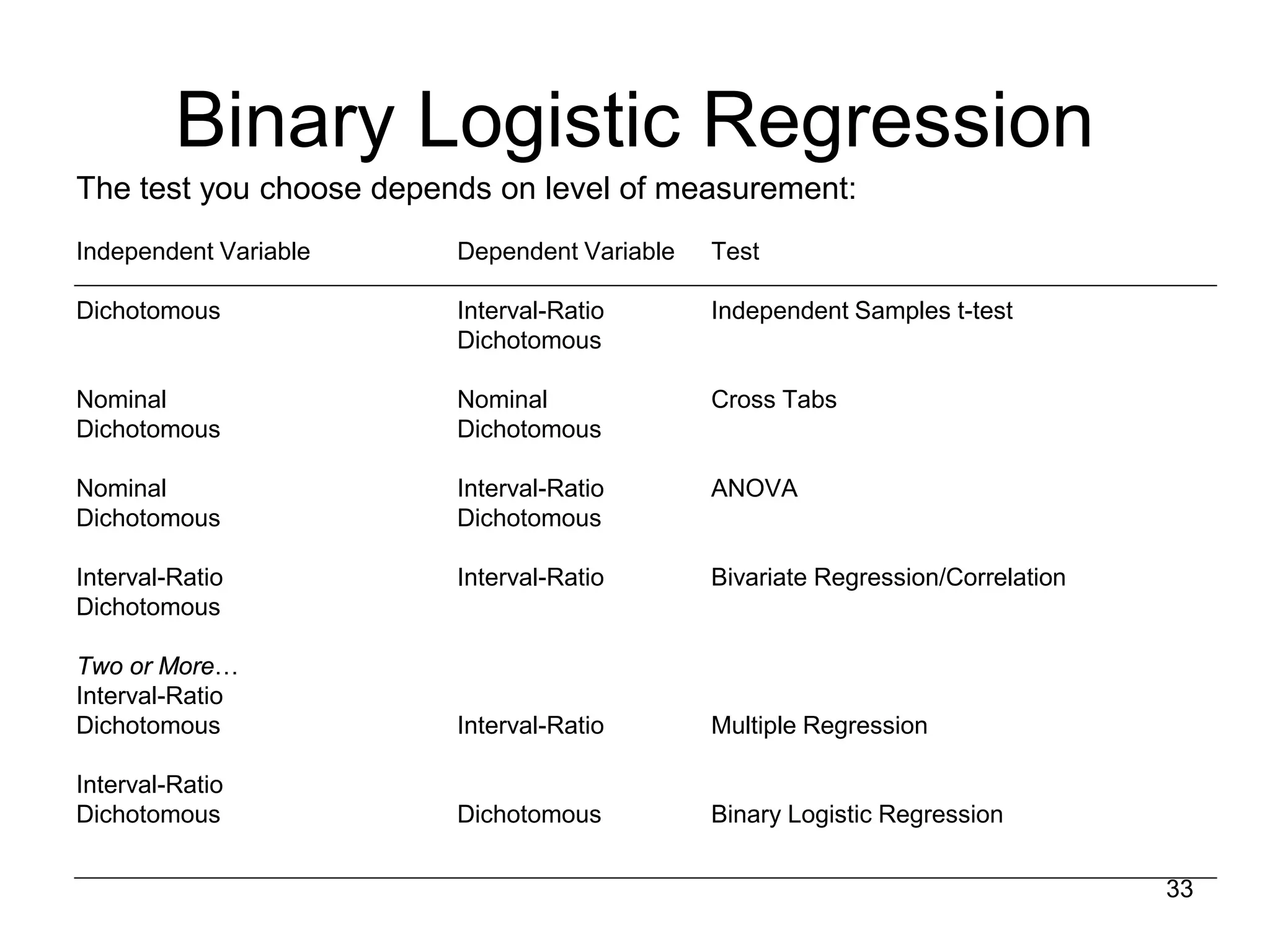
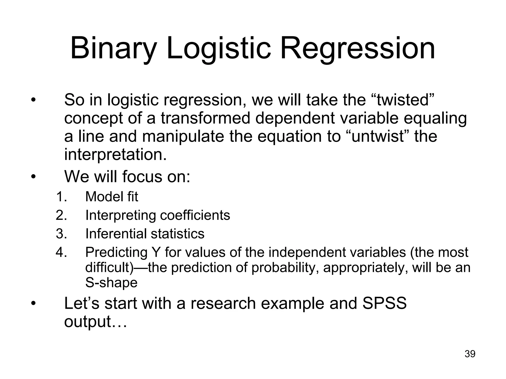
- Binary logistic regression predicts the probability of an outcome being 1 or 0 based on predictor variables. It addresses issues with ordinary least squares regression when the dependent variable is binary.
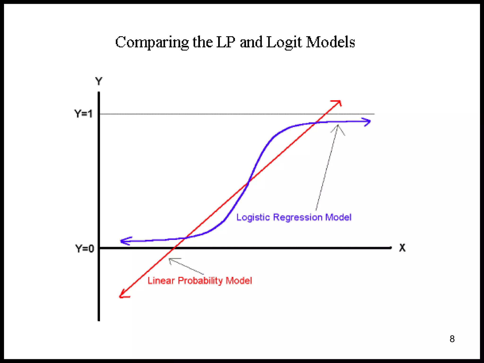
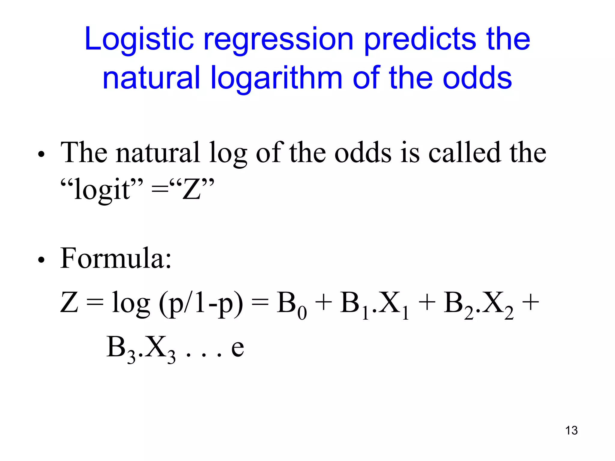
- The logistic regression model transforms the dependent variable using the logit function, ln(p/(1-p)), where p is the probability of an outcome being 1. This results in a linear relationship that can be modeled.
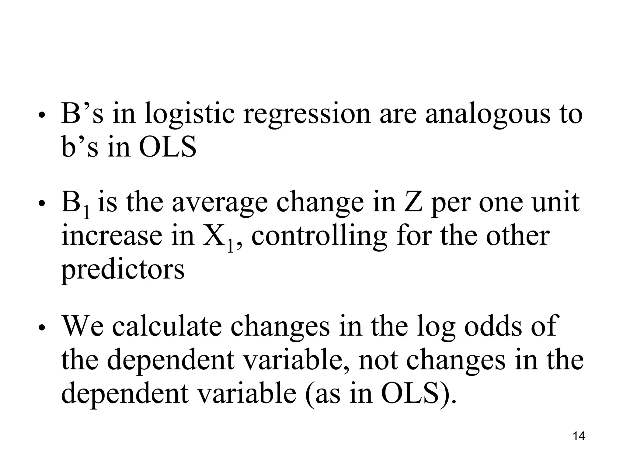
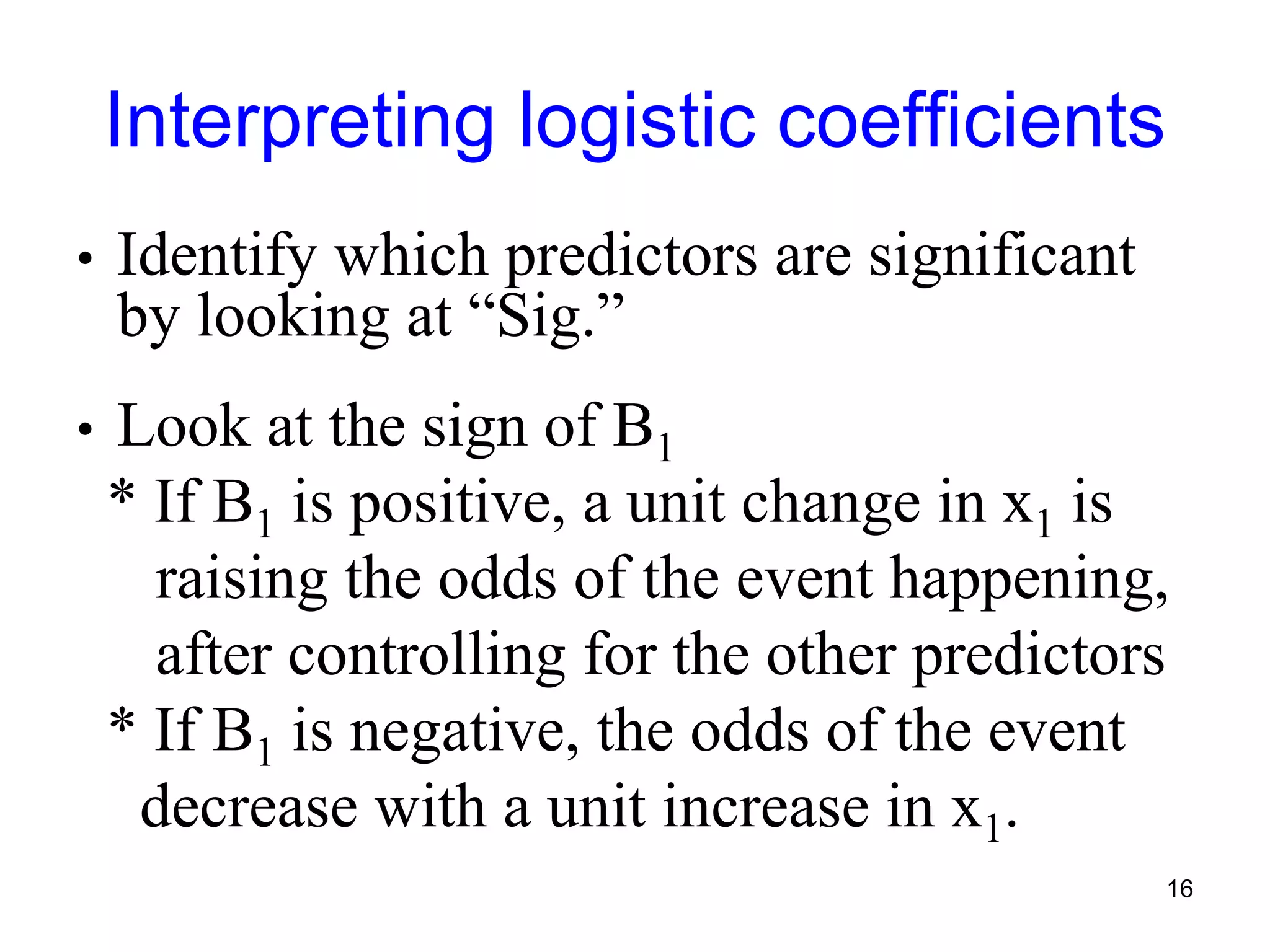
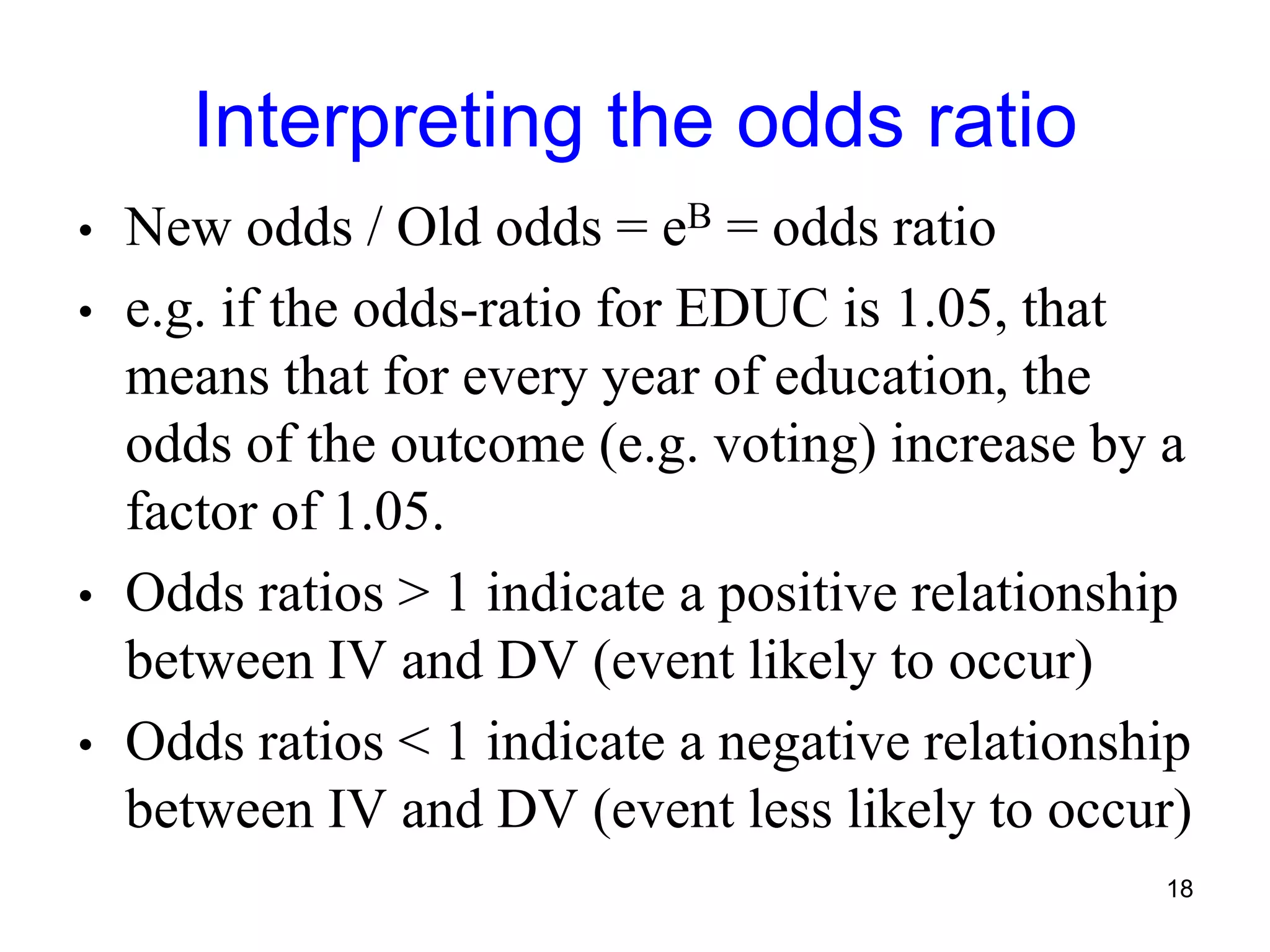
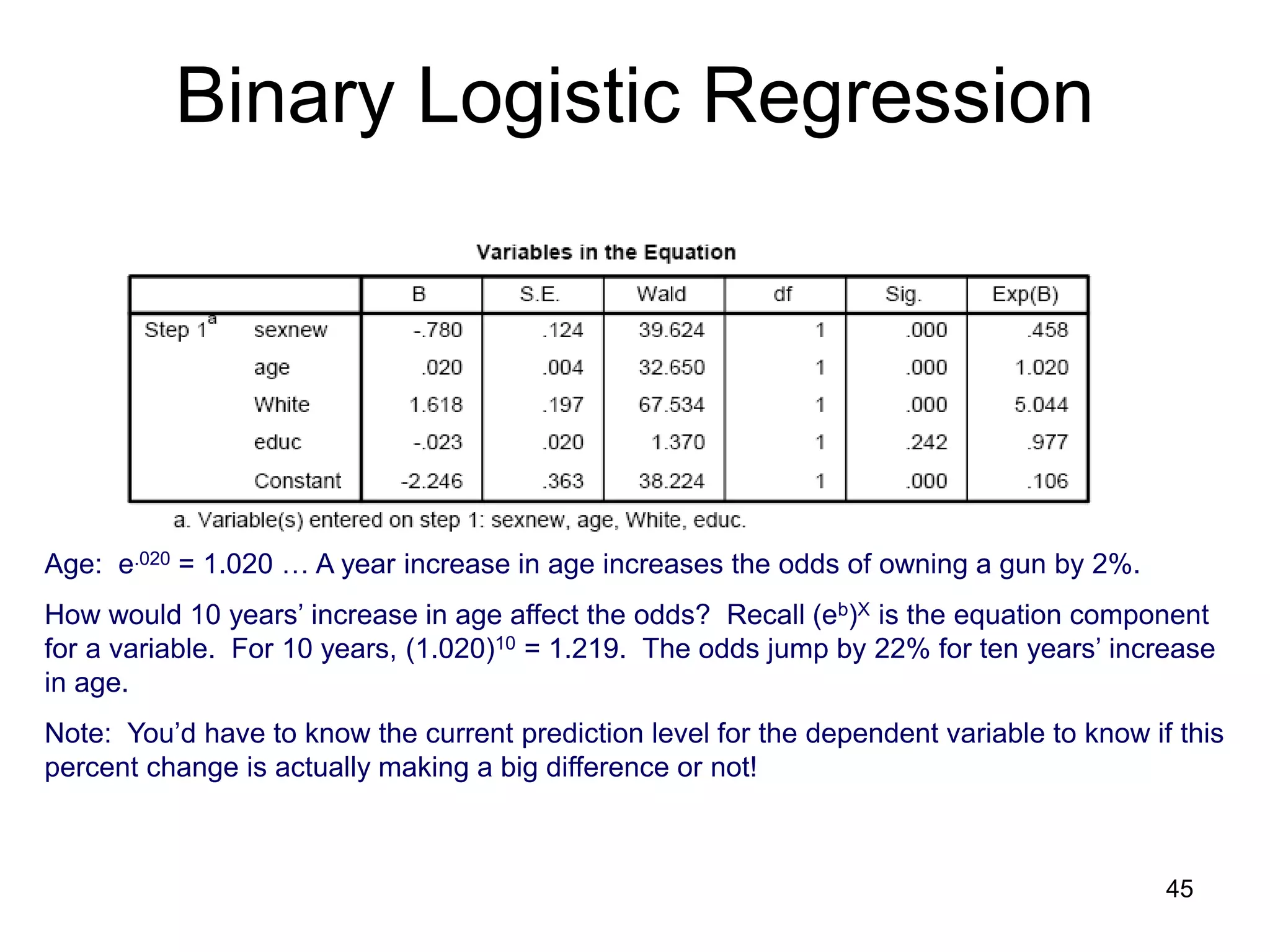
- Interpretation of coefficients is similar to ordinary least squares regression but focuses on odds ratios. A positive coefficient increases the odds of an outcome being 1, while a negative coefficient decreases the odds. The odds ratio indicates how much the odds change with a one-


![Binary Logistic Regression
• The “logit” model solves these problems:
– ln[p/(1-p)] = a + BX
or
– p/(1-p) = ea + BX
– p/(1-p) = ea (eB)X
Where:
“ln” is the natural logarithm, logexp, where e=2.71828
“p” is the probability that Y for cases equals 1, p (Y=1)
“1-p” is the probability that Y for cases equals 0,
1 – p(Y=1)
“p/(1-p)” is the odds
ln[p/1-p] is the log odds, or “logit” 6](https://image.slidesharecdn.com/regression-logistic-4-230605161759-2ff99f1a/75/Regression-Logistic-4-pdf-6-2048.jpg)
![Binary Logistic Regression
• Logistic Distribution
• Transformed, however,
the “log odds” are linear.
ln[p/(1-p)]
P (Y=1)
x
x
7](https://image.slidesharecdn.com/regression-logistic-4-230605161759-2ff99f1a/75/Regression-Logistic-4-pdf-7-2048.jpg)
![Binary Logistic Regression
• Logistic Distribution
With the logistic transformation, we’re fitting
the “model” to the data better.
• Transformed, however, the “log odds” are
linear.
P(Y = 1) 1
.5
0
X = 0 10 20
Ln[p/(1-p)]
X = 0 10 20
10](https://image.slidesharecdn.com/regression-logistic-4-230605161759-2ff99f1a/75/Regression-Logistic-4-pdf-10-2048.jpg)

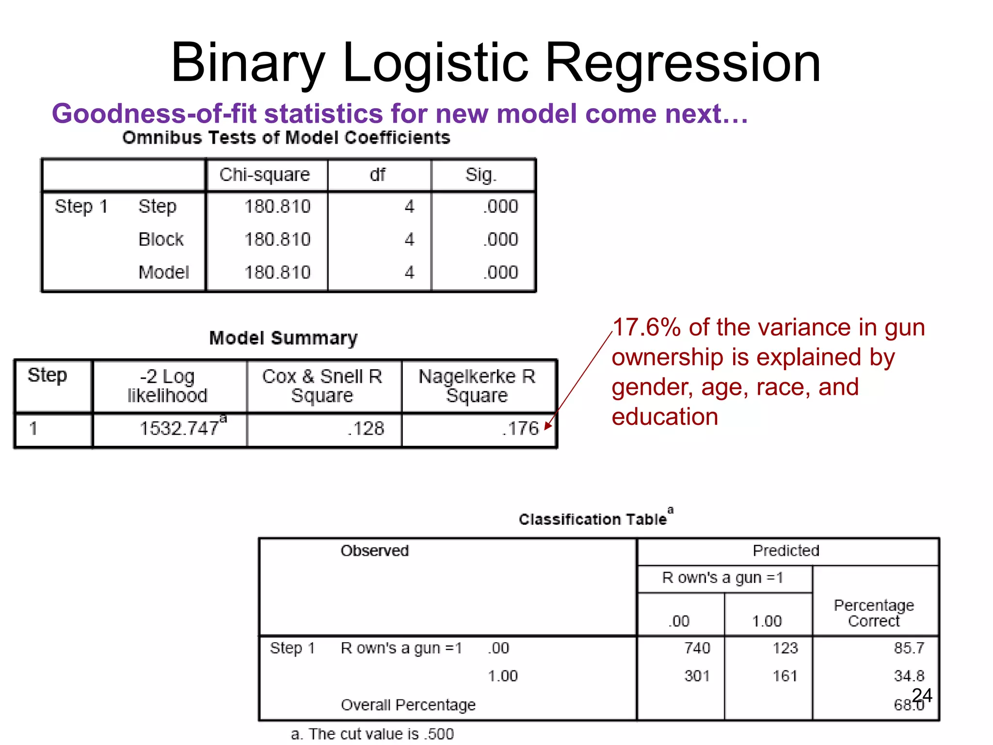
![Binary Logistic Regression
Goodness-of-fit statistics for new model come next…
Test of new model vs. intercept-
only model (the null model), based
on difference of -2LL of each. The
difference has a X2 distribution. Is
new -2LL significantly smaller?
The -2LL number is “ungrounded,” but it has a χ2
distribution. Smaller is better. In a perfect model, -2 log
likelihood would equal 0.
These are attempts to
replicate R2 using information
based on -2 log likelihood,
(C&S cannot equal 1)
-2(∑(Yi * ln[P(Yi)] + (1-Yi) ln[1-P(Yi)])
Assessment of new model’s
predictions
23](https://image.slidesharecdn.com/regression-logistic-4-230605161759-2ff99f1a/75/Regression-Logistic-4-pdf-23-2048.jpg)
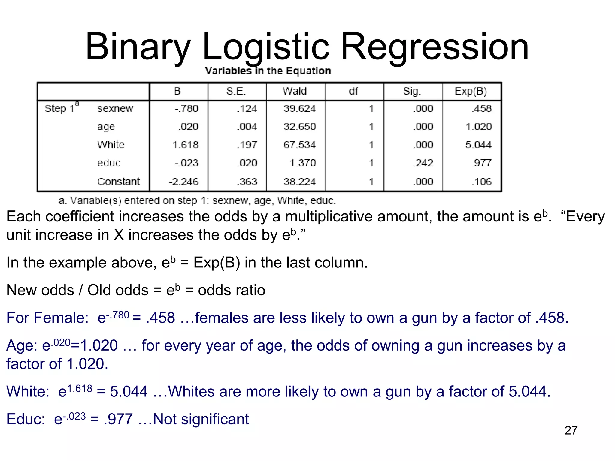
![Binary Logistic Regression
Interpreting Coefficients…
ln[p/(1-p)] = a + b1X1 + b2X2 + b3X3 + b4X4
b1
b2
b3
b4
a
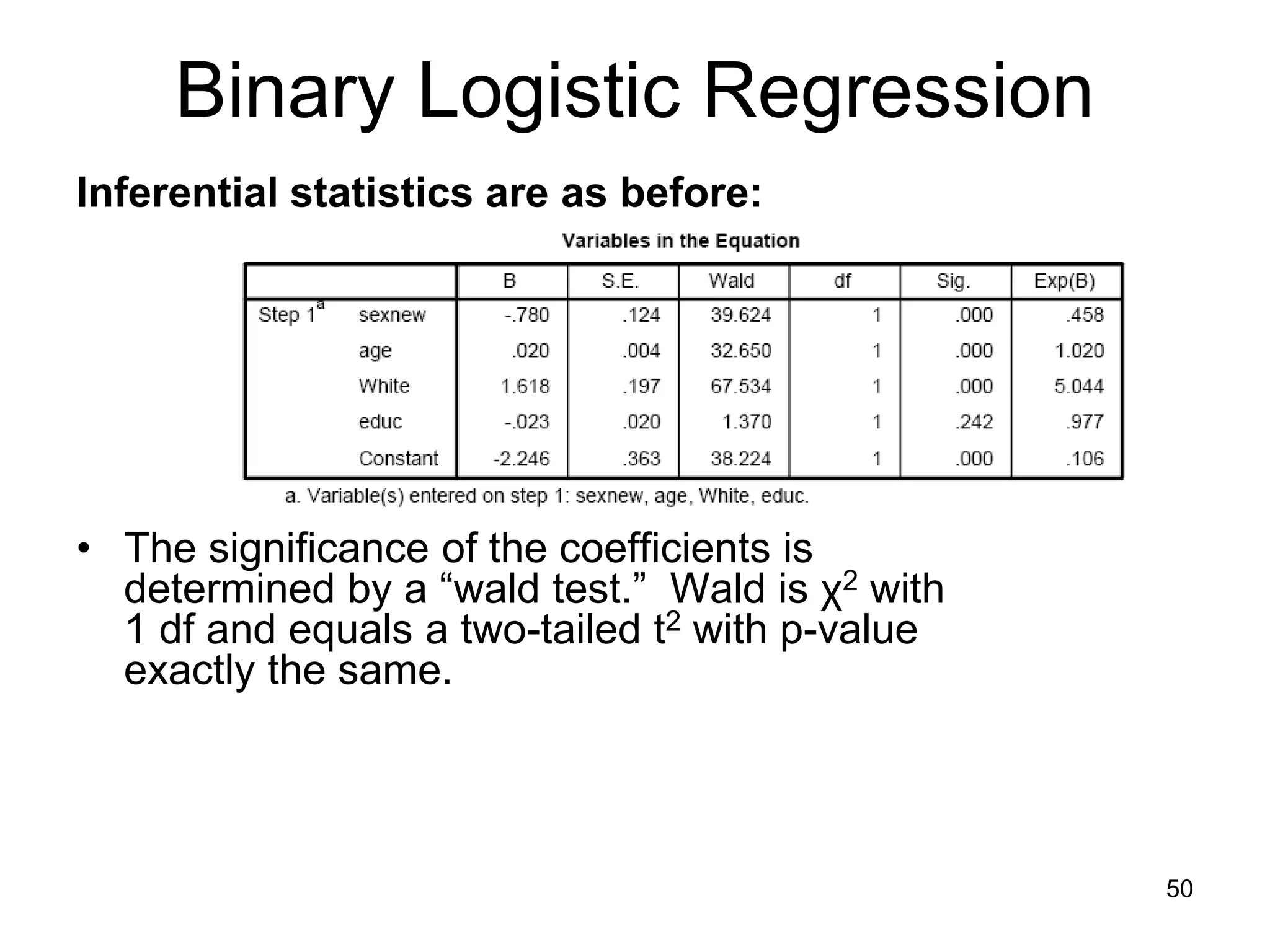
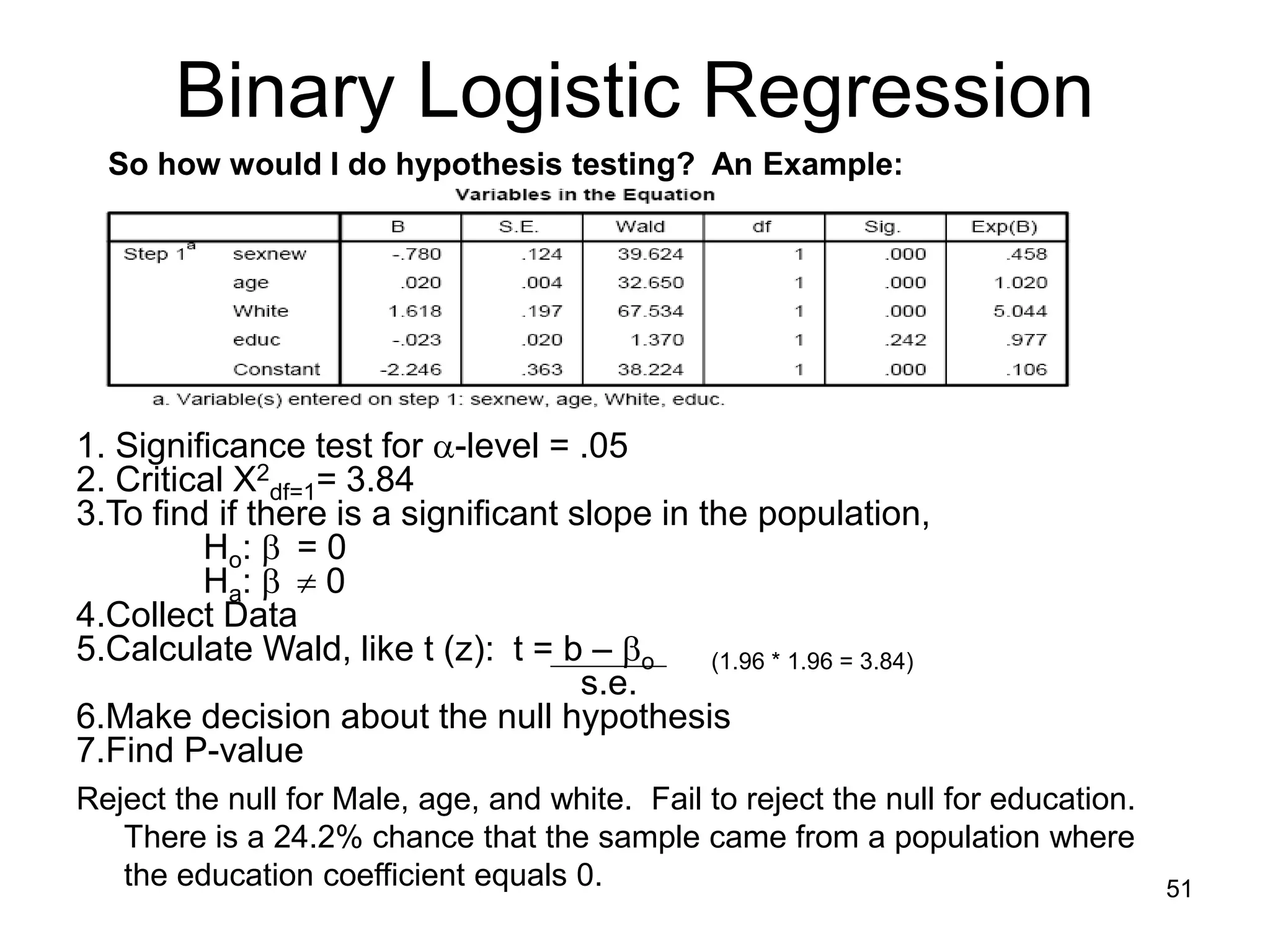
Being male, getting older, and being white have a positive effect on likelihood of
owning a gun. On the other hand, education does not affect owning a gun.
We’ll discuss the Wald test in a moment…
X1
X2
X3
X4
1
eb
Which b’s are significant?
26](https://image.slidesharecdn.com/regression-logistic-4-230605161759-2ff99f1a/75/Regression-Logistic-4-pdf-26-2048.jpg)
![Binary Logistic Regression
• So… ln[p/(1-p)] = y is same as: p/(1-p) = ey
READ THE ABOVE
LIKE THIS: when you see “ln[p/(1-P)]” say
“the value after the equal sign is
the power to which I need to take
e to get p/(1-p)”
so…
y is the power to which you
would take e to get p/(1-p)
36](https://image.slidesharecdn.com/regression-logistic-4-230605161759-2ff99f1a/75/Regression-Logistic-4-pdf-36-2048.jpg)
![Binary Logistic Regression
• So… ln[p/(1-p)] = a + bX is same as: p/(1-p) = ea + bX
READ THE ABOVE
LIKE THIS: when you see “ln[p/(1-P)]” say
“the value after the equal sign is
the power to which I need to take
e to get p/(1-p)”
so…
a + bX is the power to which you
would take e to get p/(1-p)
37](https://image.slidesharecdn.com/regression-logistic-4-230605161759-2ff99f1a/75/Regression-Logistic-4-pdf-37-2048.jpg)
![Binary Logistic Regression
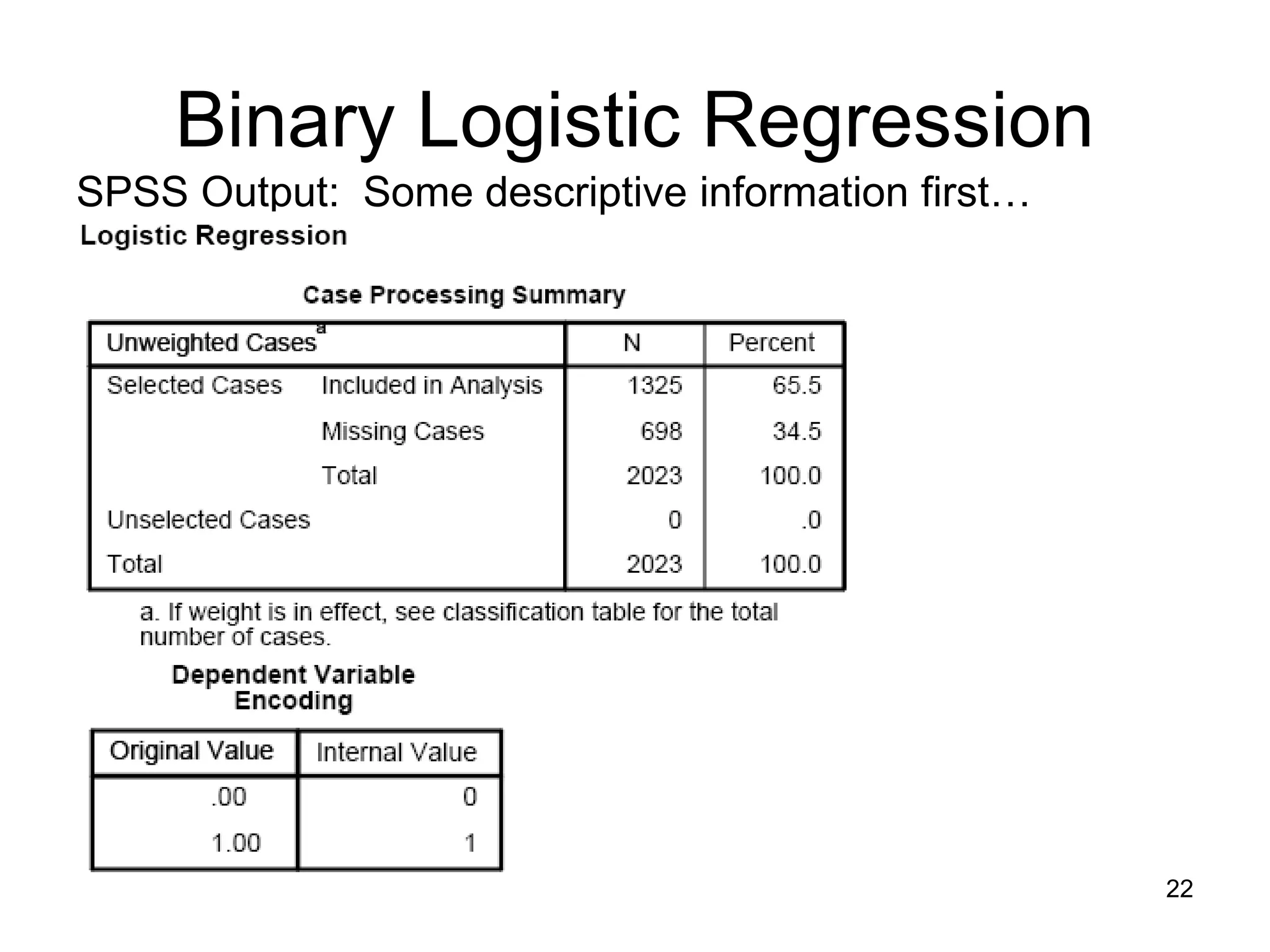
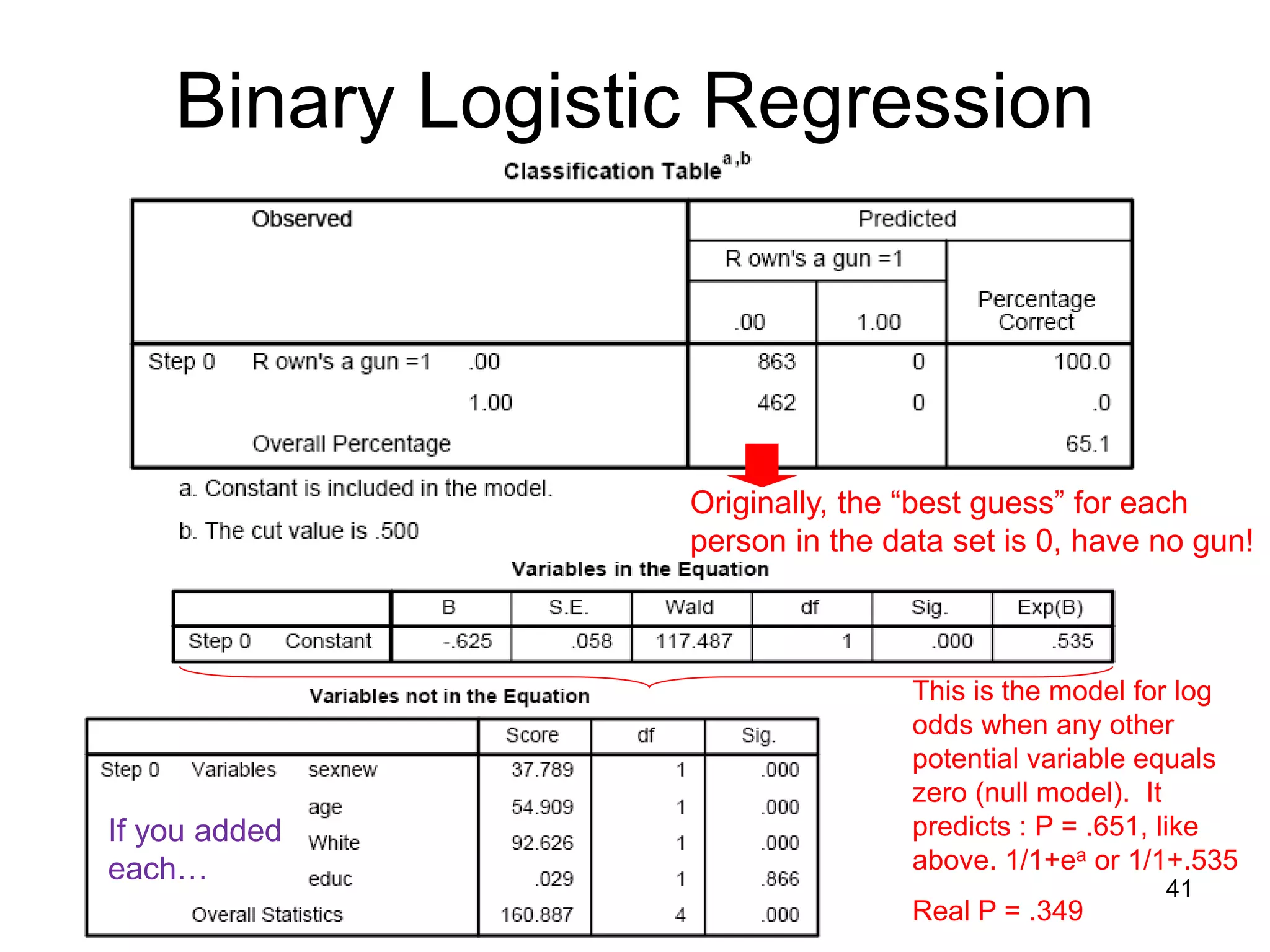
SPSS Output: Some descriptive information first…
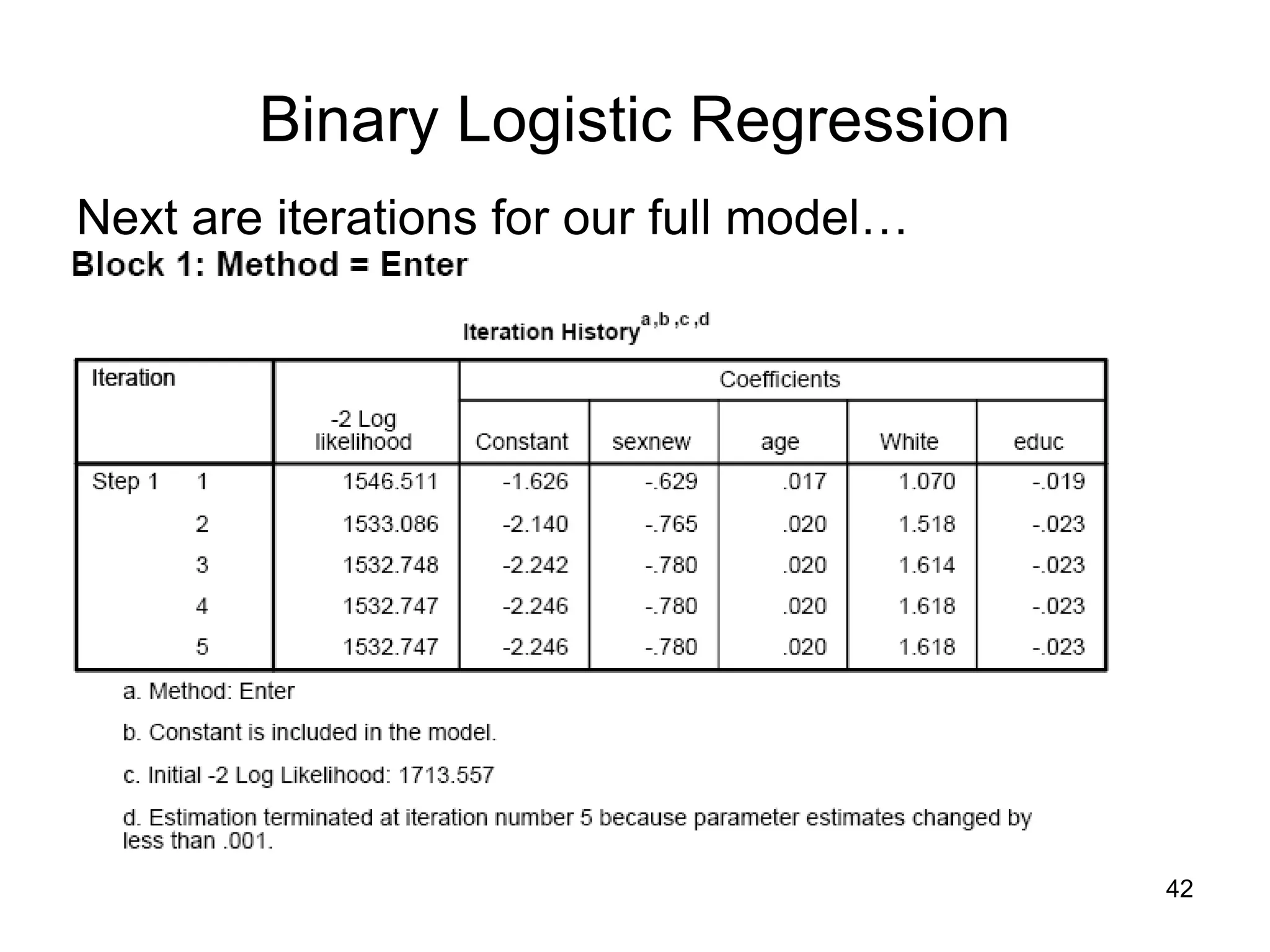
Maximum likelihood process stops at
third iteration and yields an intercept
(-.625) for a model with no
predictors.
A measure of fit, -2 Log likelihood is
generated. The equation producing
this:
-2(∑(Yi * ln[P(Yi)] + (1-Yi) ln[1-P(Yi)])
This is simply the relationship
between observed values for each
case in your data and the model’s
prediction for each case. The
“negative 2” makes this number
distribute as a X2 distribution.
In a perfect model, -2 log likelihood
would equal 0. Therefore, lower
numbers imply better model fit.
40](https://image.slidesharecdn.com/regression-logistic-4-230605161759-2ff99f1a/75/Regression-Logistic-4-pdf-40-2048.jpg)
![• ln[p/(1-p)] = a + b1X1 + …+bkXk, the power to which you
need to take e to get:
P P
1 – P So… 1 – P = ea + b1X1+…+bkXk
• Ergo, plug in values of x to get the odds ( = p/1-p).
Binary Logistic Regression
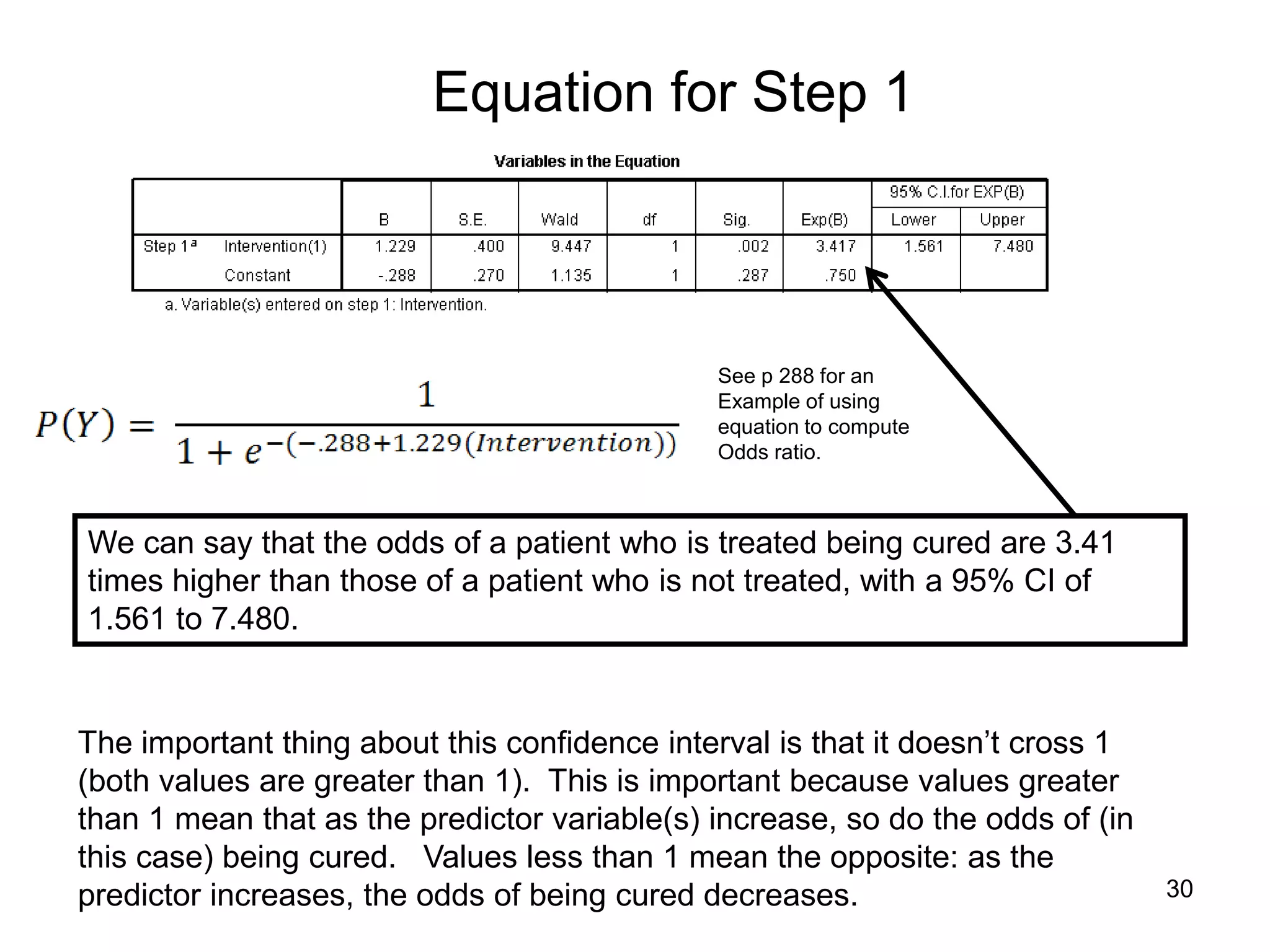
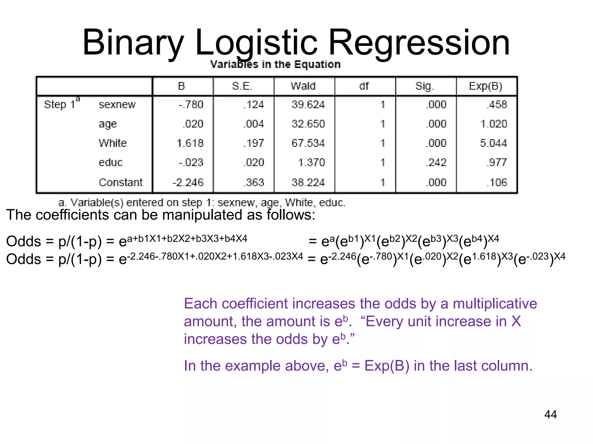
The coefficients can be manipulated as follows:
Odds = p/(1-p) = ea+b1X1+b2X2+b3X3+b4X4 = ea(eb1)X1(eb2)X2(eb3)X3(eb4)X4
Odds = p/(1-p) = ea+.898X1+.008X2+1.249X3-.056X4 = e-1.864(e.898)X1(e.008)X2(e1.249)X3(e-.056)X4
43](https://image.slidesharecdn.com/regression-logistic-4-230605161759-2ff99f1a/75/Regression-Logistic-4-pdf-43-2048.jpg)
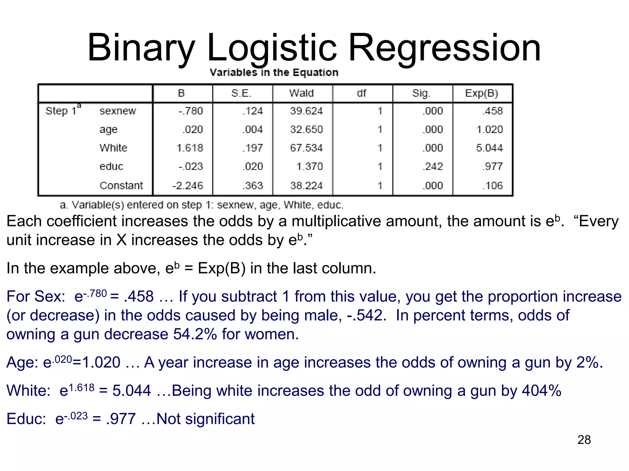
![Binary Logistic Regression
Note: You’d have to know the current prediction level for the dependent variable to
know if this percent change is actually making a big difference or not!
Recall that the logistic regression tells us two things at once.
• Transformed, the “log odds” are linear.
• Logistic Distribution
ln[p/(1-p)]
P (Y=1)
x
x
46](https://image.slidesharecdn.com/regression-logistic-4-230605161759-2ff99f1a/75/Regression-Logistic-4-pdf-46-2048.jpg)


![logistic model final_pptx__corected_one[1].pptx](https://cdn.slidesharecdn.com/ss_thumbnails/finalpptxcorectedone1-251124022241-c29356b7-thumbnail.jpg?width=640&height=640&fit=bounds)


![[DSC Europe 25] Andy Cotgreave - Nothing is new in analytics.pptx](https://cdn.slidesharecdn.com/ss_thumbnails/mba4vzcurvoh5lfrd5zw-6-251205194645-341bbbbe-thumbnail.jpg?width=640&height=640&fit=bounds)

![[DSC Europe 25] Dusan Jovicic - AI Story: From on-prem to cloud and back agai...](https://cdn.slidesharecdn.com/ss_thumbnails/8kp49m6uq22ifnbwhfnk-2-251205085715-964d11a6-thumbnail.jpg?width=640&height=640&fit=bounds)


![[DSC Europe 25] Vid Stimac - Policy Parsimony: Between Oversimplifying and Ov...](https://cdn.slidesharecdn.com/ss_thumbnails/eqlepagzqp2rhg3gbluh-dsc-stimac-251120-251205090438-059e7f54-thumbnail.jpg?width=640&height=640&fit=bounds)

![[DSC Europe 25] Bogdan Daniel Maruneac - AI - It starts with you.pptx](https://cdn.slidesharecdn.com/ss_thumbnails/odov3snhrcqs9hx5ny2n-4-251205085715-f1daacfe-thumbnail.jpg?width=640&height=640&fit=bounds)
![[DSC Europe 25] Dragan Vucic - Building the Learning Organization - How AI Tr...](https://cdn.slidesharecdn.com/ss_thumbnails/8brigo2sbu6qur6gxrra-7-251205085715-6ae07d24-thumbnail.jpg?width=640&height=640&fit=bounds)


