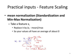
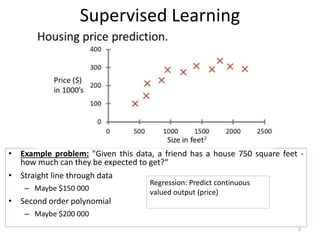
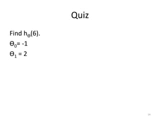
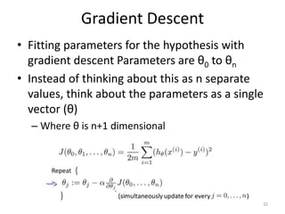
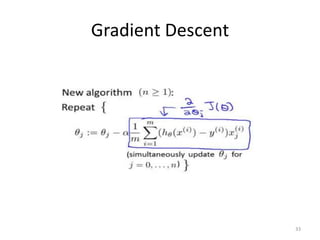
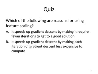
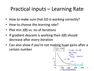
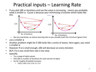
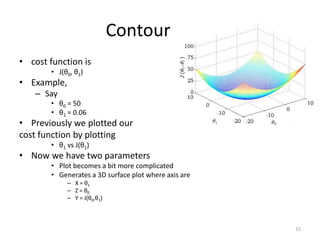
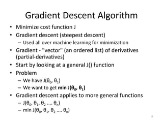
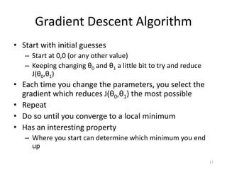
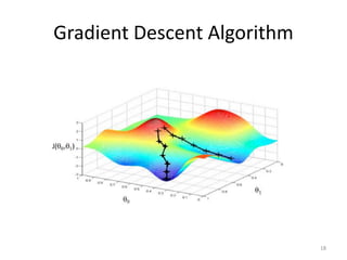
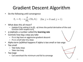
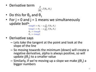
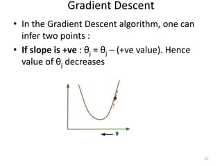
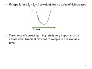
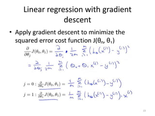
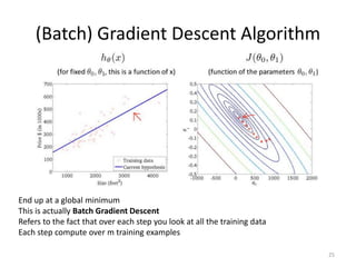
Linear regression is a supervised learning technique used to predict continuous valued outputs. It fits a linear equation to the training data to find the relationship between independent variables (x) and the dependent variable (y). Gradient descent is an algorithm used to minimize the cost function in linear regression. It works by iteratively updating the parameters (θ values) in the direction of the steepest descent as calculated by the partial derivatives of the cost function with respect to each parameter. The learning rate (α) controls the step size in each iteration. 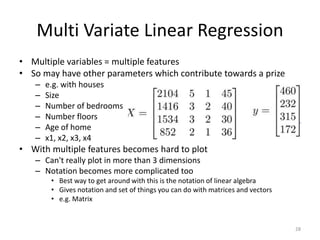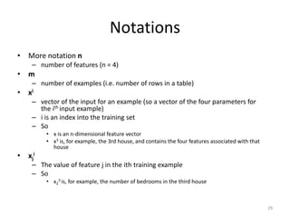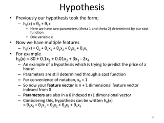Multivariate linear regression extends the technique to problems with multiple independent variables by representing the hypothesis and parameters as vectors and matrices, allowing gradient descent to optimize the parameters to fit the linear model

1. Linear Regression

2. Supervised Learning
• Example problem: "Given this data, a friend has a house 750 square feet -
how much can they be expected to get?“
• Straight line through data
– Maybe $150 000
• Second order polynomial
– Maybe $200 000
Regression: Predict continuous
valued output (price)
2

3. Supervised Learning
Classification: Discrete valued output (0 or 1)
(malignant or benign with only one attribute)
Or discrete number of possible values for the
output e.g. maybe have four values
– 0 - benign
– 1 - type 1
– 2 - type 2
– 3 - type 3
Many features to consider
• Clump thickness
• Uniformity of cell size
• Uniformity of cell shape
3

4. Regression examples

5. Linear Regression with one variable
• Housing price
• Notation m = number of training examples
• x's = input variables / features (independent)
• y's = output variable "target" variables
(dependent)
– (x,y) - single training example
– (xi, yi) - specific example (ith training example)
i is an index to training set
5

6. Linear Regression with one variable
With our training set defined - how do we use it?
• Take training set
• Pass into a learning algorithm
• Algorithm outputs a function (denoted h ) (h = hypothesis)
• This function takes an input (e.g. size of new house)
• Tries to output the estimated value of Y
6

7. Linear Regression with one variable
• How do we represent hypothesis h ?
hθ(x) = θ0 + θ1x
• What does this mean?
– Y is a linear function of x
• θi are parameters
• θ0 is zero condition
• θ1 is gradient
• This kind of function is a linear regression with
one variable is called univariate linear regression
7

8. Plots with different Ѳ0 and Ѳ1 values
8

9. • Lets us figure out how to fit the best straight line to our data
• Choosing values for θi (parameters)
– Different values give you different functions
– If θ0 is 1.5 and θ1 is 0 then we get straight line parallel with X along 1.5 @ y
• Based on our training set we want to generate parameters which make the straight
line
• Choose these parameters so that hθ(x) is close to y for our training examples
• To formalize this;
– We want to want to solve a minimization problem
– Error = hθ(x) - y
– Minimize (hθ(x) - y)2
• i.e. minimize the difference between h(x) and y for each/any/every
example
– Sum this over the training set
9
COST FUNCTION

10. • Hypothesis - is like your prediction machine,
throw in an x value, get a putative y value
• This cost function is also called the squared
error cost function
– This cost function is reasonable choice for most
regression functions
10

11. • The cost function determines parameters
• Simplified hypothesis
– Assume θ0 = 0
• Cost function and goal here are very similar to when we have θ0, but with a
simpler parameter
– Simplified hypothesis makes visualizing cost function J() a bit easier
• So hypothesis pass through 0,0
• Two key functions we want to understand
– hθ(x)
• Hypothesis is a function of x - function of what the size of the house is
– J(θ1)
• Is a function of the parameter of θ1
– So for example
• θ1 = 1
• J(θ1) = 0
– Plot
• θ1 vs J(θ1)
• Data
– 1)
» θ1 = 1
» J(θ1) = 0
– 2)
» θ1 = 0.5
» J(θ1) = ~0.58
– 3)
» θ1 = 0
» J(θ1) = ~2.3
– If we compute a range of values plot
• J(θ1) vs θ1 we get a polynomial (looks like a quadratic)
• here θ1 = 1 is the best value for θ1
11

12. 12

13. Quiz
Let
What is J(0,1)?
13
X Y
5 4
3 4
0 1
4 3

14. Quiz
Find hѲ(6).
Ѳ0= -1
Ѳ1 = 2
14

15. Contour plots
• cost function is
• J(θ0, θ1)
• Example,
– Say
• θ0 = 50
• θ1 = 0.06
• Previously we plotted our
cost function by plotting
• θ1 vs J(θ1)
• Now we have two parameters
• Plot becomes a bit more complicated
• Generates a 3D surface plot where axis are
– X = θ1
– Z = θ0
– Y = J(θ0,θ1)
15

16. Gradient Descent Algorithm
• Minimize cost function J
• Gradient descent (steepest descent)
– Used all over machine learning for minimization
• Gradient - "vector" (an ordered list) of derivatives
(partial-derivatives)
• Start by looking at a general J() function
• Problem
– We have J(θ0, θ1)
– We want to get min J(θ0, θ1)
• Gradient descent applies to more general functions
– J(θ0, θ1, θ2 .... θn)
– min J(θ0, θ1, θ2 .... θn)
16

17. Gradient Descent Algorithm
• Start with initial guesses
– Start at 0,0 (or any other value)
– Keeping changing θ0 and θ1 a little bit to try and reduce
J(θ0,θ1)
• Each time you change the parameters, you select the
gradient which reduces J(θ0,θ1) the most possible
• Repeat
• Do so until you converge to a local minimum
• Has an interesting property
– Where you start can determine which minimum you end
up
17

18. Gradient Descent Algorithm
18

19. Gradient Descent Algorithm
• Do the following until convergence
• What does this all mean?
– Update θj by setting it to (θj - α) times the partial derivative of the cost
function with respect to θj
• α (alpha)Is a number called the learning rate
• Controls how big a step you take
– If α is big have an aggressive gradient descent
– If α is small take tiny steps
• Alpha term (α)What happens if alpha is too small or too large
• Too small
– Take baby steps
– Takes too long
• Too large
– Can overshoot the minimum and fail to converge
19

20. • Derivative term
• Do this for θ0 and θ1
• For j = 0 and j = 1 means we simultaneously
update both
• Derivative says
– Lets take the tangent at the point and look at the
slope of the line
– So moving towards the minimum (down) will create a
negative derivative, alpha is always positive, so will
update j(θ1) to a smaller value
– Similarly, if we're moving up a slope we make j(θ1) a
bigger numbers
20

21. Gradient Descent
• In the Gradient Descent algorithm, one can
infer two points :
• If slope is +ve : θj = θj – (+ve value). Hence
value of θj decreases
21

22. • If slope is -ve : θj = θj – (-ve value). Hence value of θj increases
• The choice of correct learning rate is very important as it
ensures that Gradient Descent converges in a reasonable
time.
22

23. Linear regression with gradient
descent
• Apply gradient descent to minimize the
squared error cost function J(θ0, θ1)
23

24. Linear regression with gradient
descent
• How does it work? Risk of meeting different local
optimum
• The linear regression cost function is always
a convex function - always has a single minimum
– Bowl shaped
– One global optima
• So gradient descent will always converge to global optima
• In action
– Initialize values to
• θ0 = 900
• θ1 = -0.1
24

25. (Batch) Gradient Descent Algorithm
25
End up at a global minimum
This is actually Batch Gradient Descent
Refers to the fact that over each step you look at all the training data
Each step compute over m training examples

26. Quiz
Which of the following statements are true? Select
all that apply.
1. To make GD converge, we must slowly decrease
the α over time
2. GD is guaranteed to find the global minimum for
any function J(Ѳ0, Ѳ1)
3. GD can converge even if α is kept fixed
4. For the specific choice of cost function J(Ѳ0, Ѳ1)
used in LR there are no local optima (other than
global optima)
26

27. Quiz
You run gradient descent for 15 iterations with α=0.3 and
compute J(θ) after each iteration. You find that the value
J(θ) increases over time. Based on this, which of the
following conclusions seems most plausible?
1. Rather than use the current value of α, it'd be more
promising to try a larger value of α (say α=1.0).
2. α=0.3 is an effective choice of learning rate.
3. Rather than use the current value of α, it'd be more
promising to try a smaller value of α (say α=0.1).
27

28. Multi Variate Linear Regression
• Multiple variables = multiple features
• So may have other parameters which contribute towards a prize
– e.g. with houses
– Size
– Number of bedrooms
– Number floors
– Age of home
– x1, x2, x3, x4
• With multiple features becomes hard to plot
– Can't really plot in more than 3 dimensions
– Notation becomes more complicated too
• Best way to get around with this is the notation of linear algebra
• Gives notation and set of things you can do with matrices and vectors
• e.g. Matrix
28

29. Notations
• More notation n
– number of features (n = 4)
• m
– number of examples (i.e. number of rows in a table)
• xi
– vector of the input for an example (so a vector of the four parameters for
the ith input example)
– i is an index into the training set
– So
• x is an n-dimensional feature vector
• x3 is, for example, the 3rd house, and contains the four features associated with that
house
• xj
i
– The value of feature j in the ith training example
– So
• x2
3 is, for example, the number of bedrooms in the third house
29

30. Hypothesis
• Previously our hypothesis took the form;
– hθ(x) = θ0 + θ1x
• Here we have two parameters (theta 1 and theta 2) determined by our cost
function
• One variable x
• Now we have multiple features
– hθ(x) = θ0 + θ1x1 + θ2x2 + θ3x3 + θ4x4
• For example
hθ(x) = 80 + 0.1x1 + 0.01x2 + 3x3 - 2x4
– An example of a hypothesis which is trying to predict the price of a
house
– Parameters are still determined through a cost function
– For convenience of notation, x0 = 1
– So now your feature vector is n + 1 dimensional feature vector
indexed from 0
– Parameters are also in a 0 indexed n+1 dimensional vector
– Considering this, hypothesis can be written hθ(x)
= θ0x0 + θ1x1 + θ2x2 + θ3x3 + θ4x4
30

31. Hypothesis
• If we do hθ(x) =θT X
– θT is an [1 x n+1] matrix
– In other words, because θ is a column vector, the transposition
operation transforms it into a row vector
– So before
• θ was a matrix [n + 1 x 1]
– Now
• θT is a matrix [1 x n+1]
– Which means the inner dimensions of θT and X match, so they
can be multiplied together as
• [1 x n+1] * [n+1 x 1]
• = hθ(x)
• So, in other words, the transpose of our parameter vector * an input
example X gives you a predicted hypothesis which is [1 x 1]
dimensions (i.e. a single value)
31

32. Gradient Descent
• Fitting parameters for the hypothesis with
gradient descent Parameters are θ0 to θn
• Instead of thinking about this as n separate
values, think about the parameters as a single
vector (θ)
– Where θ is n+1 dimensional
32

33. Gradient Descent
33

34. • Feature Scaling is a technique to standardize the
independent features present in the data in a
fixed range.
• It is performed during the data pre-processing to
handle highly varying magnitudes or values or
units
• If feature scaling is not done, then a machine
learning algorithm tends to weigh greater values,
higher and consider smaller values as the lower
values, regardless of the unit of the values.
– Eg. Tend to consider 3000m to be greater than 5 km
34
Practical inputs - Feature Scaling

35. Practical inputs - Feature Scaling
• You should make sure the features have
a similar scale -
Means gradient descent will converge
more quickly
• e.g.
– x1 = size (0 - 2000 feet)
– x2 = number of bedrooms (1-5)
– Means the contours generated if we
plot θ1 vs. θ2 give a very tall and thin
shape due to the huge range difference
– Running gradient descent on this kind of
cost function can take a long time to find
the global minimum
35

36. Practical inputs - Feature Scaling
• mean normalization (Standardization and
Min-Max Normalization)
– Take a feature xi
• Replace it by (xi - mean)/max
• So your values all have an average of about 0
36

37. Quiz
Which of the following are reasons for using
feature scaling?
A. It speeds up gradient descent by making it require
fewer iterations to get to a good solution
B. It speeds up gradient descent by making each
iteration of gradient descent less expensive to
compute
37

38. Quiz
If xi captures the age of the house. The values of
age between 30 and 50 and the average age of
the house is 38 years. What would be the
feature assuming you use feature scaling and
mean normalization?
38

39. Practical inputs – Learning Rate
• How to make sure that GD is working correctly?
• How to choose the learning rate?
• Plot min J(θ) vs. no of iterations
• If gradient descent is working then J(θ) should
decrease after every iteration
• Can also show if you're not making huge gains after a
certain number
39

40. Practical inputs – Learning Rate
• If you plot J(θ) vs iterations and see the value is increasing - means you probably
need a smaller α - Cause is because your minimizing a function which looks like
this
– But you overshoot, so reduce learning rate so you actually reach the minimum (green line)
• use a smaller α
• Another problem might be if J(θ) looks like a series of waves. Here again, you need
a smaller α
• However If α is small enough, J(θ) will decrease on every iteration
• BUT, if α is too small then rate is too slow
• typically
– Try a range of alpha values
– Plot J(θ) vs number of iterations for each version of alpha
– Go for roughly threefold increases
• 0.001, 0.003, 0.01, 0.03. 0.1, 0.3
40

41. Quiz
Suppose a friend runs GD 3 times with α = 0.01, α = 0.1, α = 1.
A. A is α = 0.01, B is α = 0.1, C is α = 1
B. A is α = 0.1, B is α = 0.01, C is α = 1
C. A is α = 1, B is α = 0.01, C is α = 0.1
D. A is α = 1, B is α = 0.1, C is α = 0.01
A B C
41

42. Polynomial Regression
42

43. Quiz
Suppose you want to predict a house’s price as a function of size.
Your model is
hѲ(x) = Ѳ0 + Ѳ1 size + Ѳ2 √size
Suppose size ranges from 1 to 1000 sq ft. you will implement this
by fitting a model
hѲ(x) = Ѳ0 + Ѳ1 x1 + Ѳ2 x2
Finally, suppose you want to use feature scaling(without mean
normalization). Which of the choice for x1 and x2 should you
choose?
A. x1 = size, x2 = 32 √size
B. x1 = 32 *size, x2 = √size
C. x1 = size/1000, x2 = √size / 32
D. x1 = size /32, x2 = √size
43

44. Quiz
Midterm1 midterm2 Final
89 7921 96
72 5184 74
94 8836 84
69 4761 78
Using feature scaling with mean normalization,
what is the normalized feature of x1(3)?
44

45. Quiz
Suppose you have a dataset with m=1000000 examples
and n=200000 features for each example. You want to use
multivariate linear regression to fit the parameters θ to our
data. Should you prefer gradient descent or the normal
equation?
1. Gradient descent, since (XTX)−1 will be very slow to
compute in the normal equation.
2. The normal equation, since it provides an efficient way to
directly find the solution.
3. The normal equation, since gradient descent might be
unable to find the optimal θ.
4. Gradient descent, since it will always converge to the
optimal θ.
45

46. Quiz
Which of the following are reasons for using feature
scaling?
1. It speeds up gradient descent by making it require
fewer iterations to get to a good solution.
2. It speeds up gradient descent by making each
iteration of gradient descent less expensive to
compute.
3. It prevents the matrix XTX (used in the normal
equation) from being non-invertable
(singular/degenerate).
4. It is necessary to prevent the normal equation from
getting stuck in local optima.
46

47. Quiz
Which of the following plots is best suited to
test the linear relationship of independent
and dependent continuous variables?
1. Scatter Plot
2. Bar Chart
3. Histograms
4. None of the above options
47

48. Quiz
If you have only one independent variable,
how many coefficients will you require to
estimate in a simple linear regression
model?
1. One
2. Two
3. Three
4. Four
48