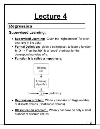
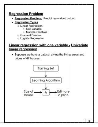
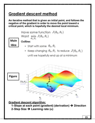
1. Regression is a supervised learning technique used to predict continuous valued outputs. It can be used to model relationships between variables to fit a linear equation to the training data. 2. Gradient descent is an iterative algorithm that is used to find the optimal parameters for a regression model by minimizing the cost function. It works by taking steps in the negative gradient direction of the cost function to converge on the local minimum. 3. The learning rate determines the step size in gradient descent. A small learning rate leads to slow convergence while a large rate may oscillate and fail to converge. Gradient descent automatically takes smaller steps as it approaches the local minimum.

1. 1
Artificial Neural
Network

2. 2
Lecture 4
Regression
Supervised Learning:
• Supervised Learning: Given the “right answer” for each
example in the data.
• Formal Definition: given a training set, to learn a function
h : X → Y so that h(x) is a “good” predictor for the
corresponding value of y.
• Function h is called a hypothesis.
• Regression problem: When y can take on large number
of discrete values (Continuous values)
• Classification problem: When y can take on only a small
number of discrete values

3. 3
Regression Problem
• Regression Problem: Predict real-valued output
• Regression Types
o Linear Regression
§ One variable
§ Multiple variables
o Gradient Descent
o Logistic Regression
Linear regression with one variable - Univariate
linear regression
• Suppose we have a dataset giving the living areas and
prices of 47 houses:

4. 4
Mathematics VS Regression
• Example-1 : Training set of housing prices

5. 5
• We can draw multiple lines to represent the data
• We need to know the best fit line for the data

6. 6
• Regression Model
• Parameters:
Regression Equation : Price = Q0 * area + Q1
Regression Equation : y = Q0 * x + Q1
Parameters : Q0 , Q1
• How to choose parameters
Ø Calculate error for each point in training data
which is the difference between the predicted value
and the correct output value

7. 7
Ø Calculate total error which is the summation for all
errors for each data point in the training set

8. 8
• Example 2 - Training set of housing prices
Notation:
m = Number of training examples
x’s = “input” variable / features
y’s = “output” variable / “target” variable
(x,y) = one training example
(x(i),y(i)) = ith training example
• We can plot this data:

9. 9
How do we represent hypothesis h(x) ?
• h(x) is a linear function with one varibale x
Parameters(Q0 , Q1) determine line position (Hypothesis)

10. 10
How to choose parameters θi‘s ?
• Error rate : the diffirence between the ouput of the
hypothesis function h(x) and the correct output of in the
training data
• we want to minimize the error rate (predicted-actual)

11. 11
Problem formulation – General Case (θ0 , θ1)
Problem formulation – Simplified case (θ1)

12. 12
How to minimize the cost function è J(θ1)
Let’s Try
Case1: Using θ1 = 1 è J(1) = 0
x y
1 1
2 2
3 3

13. 13
Case 2: Using θ1 = 0.5 è J(0.5) = 0.58

14. 14
Case 3: Using θ1 = 0 è J(0) = 2.3

15. 15
Gradient descent method
An iterative method that is given an initial point, and follows the
negative of the gradient in order to move the point toward a
critical point, which is hopefully the desired local minimum.
Gradient descent algorithm:
1-Slope at each point (gradient) (derivation) è Direction
2-Step Size è Learning rate (a)
Main
Idea
Figure

16. 16
Revised: Slope of a line
Revised: Slope of a point
è So we use derivation which is the slope of the tangent of the
curve at that point

17. 17
Revised: partial derivative of a function
Critical Point
Ø When we have a zero slope at a point x (i.e., f′(x)=0), we call x as a critical
point or a stationary point.
Ø This stationary point can either be a local minimum or a local maximum or
saddle point
Ø When the value of f(x) is lower than its value at of all the neighbors of x,
then x is called the local minimum.

18. 18
Ø if the value of f(x) is greater than its value at all the neighboring points of x,
then x is called the local maximum.
Ø If the value of f(x) is greater than some of x’s neighbors and less than some
other neighbors. Such a point is known as a saddle point.
Ø A global minima is the point where the function’s value is the minimum of all
the possible points in the domain of the function. In other words, there is no
other point x such that f(x)<f(x∗) where x∗ is the global minima of the
function f(x).
Problems of gradient descent algorithms
Local minimum : It performance Depends on the starting point of
the algorithm

19. 19
Figure of Local minimum
Gradient descent algorithm
Idea:
Update All parameters at last
Note:
gradient , slope, derivative

20. 20
Convergence – slope and direction
Update equation
1- Positive gradient (slope) è move to left direction

21. 21
2- Negative gradient (slope) è move to right direction
Learning Rate : α
1- small learning rate
2- Large learning rate

22. 22
Converge to a local minimum,
As we approach a local minimum, gradient descent will
automatically
take smaller steps. So, no need to decrease α over time.
How to compute the gradient –derivative

23. 23