Download as PPSX, PPTX
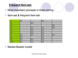
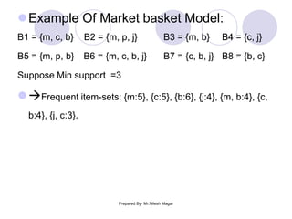
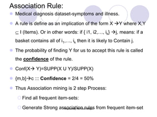
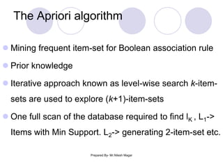
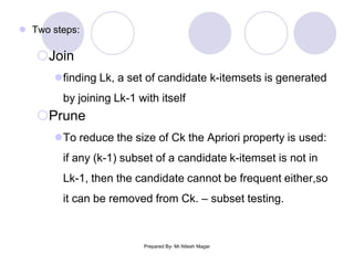


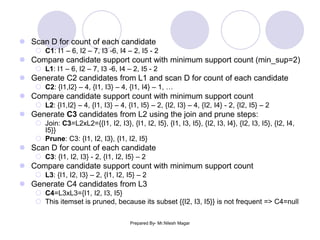
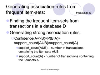

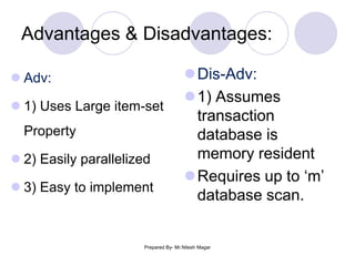
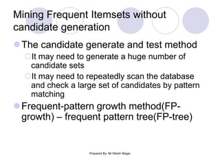
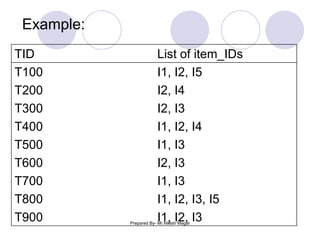
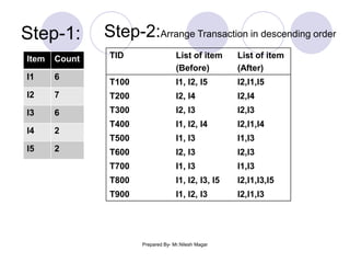
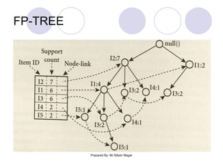

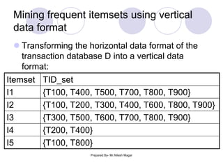


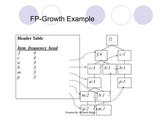
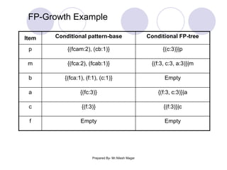
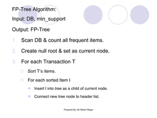

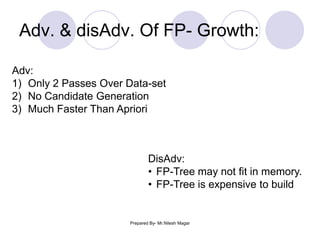


The document discusses frequent itemset mining methods. It describes the Apriori algorithm which uses a candidate generation-and-test approach involving joining and pruning steps. It also describes the FP-Growth method which mines frequent itemsets without candidate generation by building a frequent-pattern tree. The advantages of each method are provided, such as Apriori being easily parallelized but requiring multiple database scans.