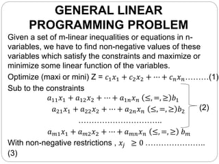
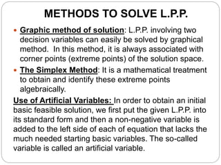
This document provides an overview of linear programming problems (LPP), including: 1) It defines the key components of an LPP as decision variables, an objective function, and constraints on available resources. 2) It describes methods for solving LPPs, including graphical and simplex methods. The simplex method algebraically identifies optimal extreme point solutions. 3) It explains some important theorems regarding LPPs, such as the fundamental theorem stating an optimal solution exists at an extreme point of the feasible region if it is finite. 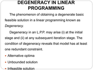4) It discusses degeneracy, which can occur when a solution has redundant constraints, and may result in alternative optima or an unbounded solution.

1. DALLY MARIA EVANGELINE A
ASSISTANT PROFESSOR OF
MATHEMATICS
BON SECOURS COLLEGE FOR
WOMEN
THANJAVUR, TAMIL NADU
LINEAR PROGRAMMING PROBLEM

2. OPERATIONS RESEARCH
 O.R. is the application of scientific methods,
techniques and tools to problems involving the
operations of a system so as to provide those in
control of the system with optimum solutions to
the problem.
 It is a scientific knowledge through
interdisciplinary team effort for the purpose of
determining the best utilizing of limited resources.

3. LINEAR PROGRAMMING
PROBLEM
 Linear Programming Problem, abbreviated as L.P.P.,
is a technique for determining an optimum schedule
of interdependent activities in view of the available
resources.
 Programming, is just another word for “planning” and
refers to the process of determining a particular plan
of action from amongst several alternatives.
 The word linear stands for indicating that all
relationships involved in a particular problem are
linear.

4. COMPONENTS OF LPP
A Linear Programming Problem consists of three components,
namely decision variables, objective and constraints
(restrictions).
 The decision variables refers to the activities that are
competing one another for sharing the resources available.
All the decision variables are considered as continuous,
controllable and non – negative.
 A linear programming problem must have an objective
which should be clearly identifiable and measurable in
quantitative terms.
 There are always certain limitations (or conditions,
constraints) on the use of resources, such as labour, space,

5. GENERAL LINEAR
PROGRAMMING PROBLEM
Given a set of m-linear inequalities or equations in n-
variables, we have to find non-negative values of these
variables which satisfy the constraints and maximize or
minimize some linear function of the variables.
Optimize (maxi or mini) Z = 𝑐1 𝑥1 + 𝑐2 𝑥2 + ⋯ + 𝑐 𝑛 𝑥 𝑛………(1)
Sub to the constraints
𝑎11 𝑥1 + 𝑎12 𝑥2 + ⋯ + 𝑎1𝑛 𝑥 𝑛 ≤, =, ≥ 𝑏1
𝑎21 𝑥1 + 𝑎22 𝑥2 + ⋯ + 𝑎2𝑛 𝑥 𝑛 ≤, =, ≥ 𝑏2
…………………………..
𝑎 𝑚1 𝑥1 + 𝑎 𝑚2 𝑥2 + ⋯ + 𝑎 𝑚𝑛 𝑥 𝑛 ≤, =, ≥ 𝑏 𝑚
With non-negative restrictions , 𝑥𝑗 ≥ 0 …………………..
(3)
(2)

6. SOLUTIONS OF LPP
 Solution: The values of the variables 𝑥𝑗
′
𝑠, (𝑗 =
1, 2, … 𝑛), that satisfies the equation (2) is called
solution to the given LPP.
 Feasible solution: A solution that satisfies the
equation (3), that is, the non – negativity
restriction is called feasible solution of the given
LPP.
 Optimal solution: A feasible solution that
optimizes the objective function (1) is called an
optimal solution of the given LPP.

7. CONVERSION OF INEQUALITY
INTO EQUALITY
 Slack variable: A positive variable added to the LHS
of the constraints (2) of the given LPP in order to
convert the (≤) “less than or equal to” type constraint
into an equation is called an slack variable.
 Surplus variable: A positive variable subtracted from
the LHS of the constraints(2) of the given LPP in
order to convert the (≥) “greater than or equal to”
type constraint into an equation is called an surplus
variable.

8. SIMULTANEOUS LINEAR
EQUATIONS
Given m-simultaneous linear equations in n unknown
(m<n).
Given 𝐴 𝑥 = 𝑏
𝑗=1
𝑛
𝑎𝑖𝑗 𝑥𝑗 = 𝑏𝑖, (𝑖 = 1,2, … , 𝑚)
where 𝐴 = [𝑎𝑖𝑗] 𝑚×𝑛 , 𝑏 = [𝑏1, 𝑏2, … . , 𝑏 𝑚] and 𝑥 =
[𝑥1, 𝑥2, … , 𝑥 𝑛]. Let 𝐴 is an 𝑚 × 𝑛 matrix of rank m. Let 𝑏 be a
column matrix of m rows.
Degeneracy: A basic solution to 𝐴 𝑥 = 𝑏 is degenerate if
one or more of the basic variables vanish.

9. SOME IMPORTANT RESULTS
 A necessary and sufficient condition for the existence
and non – degeneracy of all possible basic solutions of
𝐴 𝑥 = 𝑏 is the linear independence of every set of m
columns from the augmented matrix 𝐴 𝑏 = ( 𝐴, 𝑏).
 A necessary and sufficient condition for any given
basic solution 𝑥 𝐵 = 𝐵−1
𝑏 to be non-degenerated is
the linear independence of 𝑏 and every set of (m-1)
columns from 𝐵.

10. SOME IMPORTANT THEOREMS
 If a linear programming problem has a feasible
solution then it also has a basic feasible solution.
 There exists only finite number of basic feasible
solutions to linear programming problem.
 If a linear programming problem have a basic feasible
solution and we drop one of the basic vector and
introduce a non-basic vector in the basis set, then the
new solution obtained is also a basic feasible solution.
 Any convex combination of k-different optimum
solution to a linear programming problem is again an
optimum solution to the problem.

11. GEOMETRIC INTERPRETATION
OF L.P.P.
Whenever the feasible solution of linear
programming problem exists, the region of feasible
solution is a convex set and there also exist
extreme points. If the optimal solution exists one of
the extreme point is optimal.
Whenever the optimal value of objective
function Z is finite, at least one extreme point of the
region of feasible solution has an optimal solution.
If optimal solution is not unique, there are points
other than extreme points that were optimal, but in
any case one extreme point is optimal.

12. METHODS TO SOLVE L.P.P.
 Graphic method of solution: L.P.P. involving two
decision variables can easily be solved by graphical
method. In this method, it is always associated with
corner points (extreme points) of the solution space.
 The Simplex Method: It is a mathematical treatment
to obtain and identify these extreme points
algebraically.
Use of Artificial Variables: In order to obtain an initial
basic feasible solution, we first put the given L.P.P. into
its standard form and then a non-negative variable is
added to the left side of each of equation that lacks the
much needed starting basic variables. The so-called
variable is called an artificial variable.

13. SOME IMPORTANT
THEOREMS
 FUNDAMENTAL THEOREM OF LINEAR
PROGRAMMING:
If the feasible region of an L.P.P. is a convex
polyhedron, then there exists an optimal solution to the
L.P.P. and at least one basic feasible solution must be
optimal.
 UNBOUNDED SOLUTION:
Let there exist a basic feasible solution to a given
L.P.P. If for at least one j, for which 𝑦𝑖𝑗 ≤ 0 (i =

14. DEGENERACY IN LINEAR
PROGRAMMING
The phenomenon of obtaining a degenerate basic
feasible solution in a linear programming known as
Degeneracy.
Degeneracy in an L.P.P. may arise (i) at the initial
stage and (ii) at any subsequent iteration stage. The
condition of degeneracy reveals that model has at least
one redundant constraint.
 Alternative optima
 Unbounded solution
 Infeasible solution