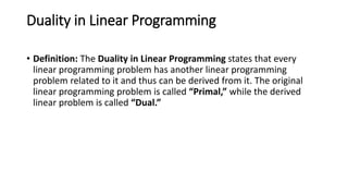
Unit 2
Linear programming and transportation problem
What is Linear Programming?
• Linear programming (LP) or Linear Optimisation may be defined as
the problem of maximizing or minimizing a linear function that is
subjected to linear constraints. The constraints may be equalities or
inequalities. The optimisation problems involve the calculation of
profit and loss.
• In other words, linear programming is considered as an optimization
method to maximize or minimize the objective function of the given
mathematical model with the set of some requirements which are
represented in the linear relationship. The main aim of the linear
programming problem is to find the optimal solution.
• Linear programming is the method of considering different
inequalities relevant to a situation and calculating the best value that
is required to be obtained in those conditions. Some of the
assumptions taken while working with linear programming are:
• The number of constraints should be expressed in the quantitative
terms
• The relationship between the constraints and the objective function
should be linear
• The linear function (i.e., objective function) is to be optimised
Components of Linear Programming
• The basic components of the LP are as follows:
• Decision Variables
• Constraints
• Data
• Objective Functions
Mathematically, the general linear programming problem (LPP) may be stated as follows.
Maximize or Minimize Z = c1 x1 + c2 x2 + … + cn xn
Subject to the conditions (constraints)
Objective function:
A function Z=c1 x1 + c2x2 + …+ cnxn which is to be optimized (maximized or minimized) is called objective function.
Decision variable:
The decision variables are the variables, which has to be determined xj , j = 1,2,3,…,n, to optimize the objective function.
Constraints:
There are certain limitations on the use of limited resources called constraints.
Feasible solution:
A set of values of the decision variables that satisfies all the constraints of the problem and non-negativity restrictions
is called a feasible solution of the problem.
Optimal solution:
Any feasible solution which maximizes or minimizes the objective function is called an optimal solution.
Feasible region:
The common region determined by all the constraints including non-negative constraints xj ≥0 of a linear programming problem is
called the feasible region (or solution region) for the problem.
Characteristics of Linear Programming
• The following are the five characteristics of the linear programming problem:
• Constraints – The limitations should be expressed in the mathematical form, regarding
the resource.
• Objective Function – In a problem, the objective function should be specified in a
quantitative way.
• Linearity – The relationship between two or more variables in the function must be
linear. It means that the degree of the variable is one.
• Finiteness – There should be finite and infinite input and output numbers. In case, if the
function has infinite factors, the optimal solution is not feasible.
• Non-negativity – The variable value should be positive or zero. It should not be a
negative value.
• Decision Variables – The decision variable will decide the output. It gives the ultimate
solution of the problem. For any problem, the first step is to identify the decision
variables.
Linear Programming Applications
• Engineering – It solves design and manufacturing problems as it is
helpful for doing shape optimisation
• Efficient Manufacturing – To maximise profit, companies use linear
expressions
• Energy Industry – It provides methods to optimise the electric power
system.
• Transportation Optimisation – For cost and time efficiency.
The advantages of linear programming are:
• Linear programming provides insights to the business problems
• It helps to solve multi-dimensional problems
• According to the condition change, LP helps in making the
adjustments
• By calculating the cost and profit of various things, LP helps to take
the best optimal solution
Linear programming problem(LPP)
Methods to solve it
• Simplex method
• Graphical Method
Simplex Method
• Simplex method is an approach to solving linear programming models
by hand using slack variables, tableaus, and pivot variables as a
means to finding the optimal solution of an optimization problem.
• Simplex tableau is used to perform row operations on the linear
programming model as well as for checking optimality.
Terminology in Simplex Method
1. Standard Form: A LPP in which all constraints are written in
equalities.
2. Slack Variable: A variable added to the LHS of “less than or equal to”
constraint to convert the convert the constraint into an equality. Value
of slack variable indicates unused resources.
3. Surplus Variable: A variable subtracted from the LHS of “more than
or equal to” constraint to convert the convert the constraint into an
equality. Value of surplus variable indicates consumption over & above
minimum requirements.
4. Simplex Tableau: A table used to keep record of the calculation made at
each iteration.
5. Basis: The set of variables which are not restricted to equal zero in the
current basic solution. The variables which make up the basis are called Basic
variables. The remaining are called non-basic variables.
6. Iteration: The steps performed in simplex method to progress form one
feasible solution to another.
7. Cj Row: A row in the simplex table which contains the coefficients (unit
profit) of the variables in the Objective function.
8. Zj Row: A row in the simplex tables whose elements represent the
increase / decrease in the value of objective function; if one unit of that
variable is brought into the solution.
9. Zj – Cj Row (Index Row): A row in the simplex table whose elements
represent net contribution / loss per unit if one unit of that variable is
brought into the solution.
10. Key column: The column with the largest positive / negative index
number. It indicates the Entering variable in the Basis.
11. Key row: The row with the smallest positive ratio found by
dividing Quantity column values by Key column values for each row. It
indicates the Exiting variable from the Basis.
12. Key element: The element at the intersection of Key row & Key
column.
13.Decision Variables: The unknowns to be determined.
14. Constraints: Mathematical equations of the limitations imposed by the
situation or problem characteristics. Constraints define limits within which
the solution of the Problem has to be found.
15.Objective Function: The mathematical equation of the major goal of the
Problem.
16.Linear Relationship: Each Variable appears in only one term & only the
first power.
17.Feasible Solution: A set of values of Decision Variables which satisfy all
the constraints.
18.Optimal Solution: A Feasible Solution which optimizes the Objective
Function.
19.Optimality condition: The entering variable in a maximization
(minimization) problem is the non-basic variable having the most
negative (positive) coefficient in the Z-row. The optimum is reached at
the iteration where all the Z-row coefficient of the non-basic variables
are non-negative (non-positive).
20.Feasibility condition: For both maximization and minimization
problems the leaving variable is the basic associated with the smallest
non-negative ratio (with strictly positive denominator).
The steps of the simplex method
• Step 1: Determine a starting basic feasible solution.
• Step 2: Select an entering variable using the optimality condition.
Stop if there is no entering variable.
• Step 3: Select a leaving variable using the feasibility condition.
The Graphical Method
• Step 1: Formulate the LP (Linear programming) problem
• Step 2: Construct a graph and plot the constraint lines
• The graph must be constructed in ‘n’ dimensions, where ‘n’ is the number of decision variables.
This should give you an idea about the complexity of this step if the number of decision variables
increases.
• Step 3: Determine the valid side of each constraint line
• This is used to determine the domain of the available space, which can result in a feasible
solution.
• Step 4: Identify the feasible solution region
• The feasible solution region on the graph is the one which is satisfied by all the constraints. It
could be viewed as the intersection of the valid regions of each constraint line as well. Choosing
any point in this area would result in a valid solution for our objective function.
• Step 5: Plot the objective function on the graph
• It will clearly be a straight line since we are dealing with linear equations here. One must be sure
to draw it differently from the constraint lines to avoid confusion.
• Step 6: Find the optimum point
• Optimum Points
• An optimum point always lies on one of the corners of the feasible region.
• If the goal is to minimize the objective function, find the point of contact of
the ruler with the feasible region, which is the closest to the origin. This is
the optimum point for minimizing the function.
• If the goal is to maximize the objective function, find the point of contact of
the ruler with the feasible region, which is the farthest from the origin. This
is the optimum point for maximizing the function.
Terminology in graphical method
• Optimization problem: A problem that seeks to maximization or
minimization of variables of linear inequality problem is called optimization
problems.
• Feasible region: A common region determined by all given issues including
the non-negative (x ≥ 0, y ≥ 0) constrain is called the feasible region (or
solution area) of the problem. The region other than the feasible region is
known as the infeasible region.
• Feasible Solutions: These points within or on the boundary region
represent feasible solutions of the problem. Any point outside the scenario
is called an infeasible solution.
• Optimal(most feasible) solution: Any point in the emerging region that
provides the right amount (maximum or minimum) of the objective
function is called the optimal solution.
• Objective function: The direct function of form Z = ax + by, where a
and b are constant, which is reduced or enlarged is called the
objective function. For example, if Z = 10x + 7y. The variables x and y
are called the decision variable.
• Constraints: The restrictions that are applied to a linear inequality are
called constraints.
• Non-negative constraints: x > 0, y > 0 etc.
• General constraints: x + y > 40, 2x + 9y ≥ 40 etc.
• Redundant Constraint
• It is a constraint that does not affect the feasible region.
• Example: Consider the linear programming problem:
• Maximize 1170 x1 + 1110x2
• subject to
• 9x1 + 5x2 ≥ 500
7x1 + 9x2 ≥ 300
5x1 + 3x2 ≤ 1500
7x1 + 9x2 ≤ 1900
2x1 + 4x2 ≤ 1000
• x1, x2 ≥ 0
• The feasible region is indicated in the following figure:
• The critical region has been formed by the two constraints.
• 9x1 + 5x2 ≥ 500
7x1 + 9x2 ≤ 1900
• x1, x2 ≥ 0
• The remaining three constraints are not affecting the feasible region
in any manner. Such constraints are called redundant constraints.
• Degenerate Solution: A basic solution to the system of equations is
called degenerate if one or more of basic variables become equal to
zero.
Corner point method
• Identify each of the corner (or extreme points) of the feasible region
either by visual inspection or method of simultaneous equations.
• Compute profit/cost at each corner point by substituting the
coordinates of that point into the objective function.
• Identify the optimal solution at that corner point which shows the
highest profit (in maximization problem) or lowest cost ( in
minimization problem)
Iso profit or iso cost method
• In this choose a specific point or cost figure and draw iso profit or iso
cost line so that it falls within shaded region.
• Move this iso profit or iso cost line parallel to itself and farther(closer)
from (to) the origin until it takes it into feasible region.
• Identify the optimal solution as the coordinates of that point on the
feasible region touched by the highest possible iso profit line (or
lowest possible iso cost line)
• Identify coordinates of optimal point
• Compute optimal value
Duality in Linear Programming
• Definition: The Duality in Linear Programming states that every
linear programming problem has another linear programming
problem related to it and thus can be derived from it. The original
linear programming problem is called “Primal,” while the derived
linear problem is called “Dual.”
Rules for Constructing the Dual from the Primal (or primal from the dual) are:
1.If the objective of one problem is to be maximized, the objective of the other is to be minimized.
2.The Maximization problem should have all constraints and the minimization problem has all constraints
3.All primal and dual variables must be non-negative (0)
4.The elements of right hand side of the constraints in one problem are the respective coefficients of the objective function in the other problem.
5.The matrix of constraints coefficients for one problem is the transpose of the matrix of constraint coefficient for the other problem.
Characteristics of the dual problem
1. Dual of the dual is primal.
2. If either the primal of dual problem has a solution, then the other also
has a solution and their optimum values are equal.
3. If any of the two problems has only an infeasible solution then the
value of the objective function of the other is unbounded.
4. The value of the objective function for any feasible solution of the
primal is less than value of the objective function for any feasible solution of
the dual.
5. If either the primal or the dual problem has an unbounded solution
then the solution to the other problem is infeasible.
6. If the primal has a feasible solution but the dual does not have, then
the primal will not have a finite optimum solution and vice-versa.
Advantages of Duality
1. It yields a number of powerful theorems.
2. Computational procedure can be considerably reduced by converting it
into dual if the primal problem contains a large number of rows (constraints)
and a smaller number of columns (variables).
3. Solution of the dual checks the accuracy of the primal solution for
computational errors.
4. Gives additional information as to how the optimum solution changes as a
result of the changes in the coefficients and the formulation of the problem
(this is termed as post opimality or sensitivity analysis)
5. Indicates that fairly close relationships exits between linear programming
duality.
6. Economic interpretation of the dual helps the management m making
future decisions.
Unit 2.pptx
Unit 2.pptx

Unit 2.pptx

  • 1.
    Unit 2 Linear programmingand transportation problem
  • 2.
    What is LinearProgramming? • Linear programming (LP) or Linear Optimisation may be defined as the problem of maximizing or minimizing a linear function that is subjected to linear constraints. The constraints may be equalities or inequalities. The optimisation problems involve the calculation of profit and loss. • In other words, linear programming is considered as an optimization method to maximize or minimize the objective function of the given mathematical model with the set of some requirements which are represented in the linear relationship. The main aim of the linear programming problem is to find the optimal solution.
  • 3.
    • Linear programmingis the method of considering different inequalities relevant to a situation and calculating the best value that is required to be obtained in those conditions. Some of the assumptions taken while working with linear programming are: • The number of constraints should be expressed in the quantitative terms • The relationship between the constraints and the objective function should be linear • The linear function (i.e., objective function) is to be optimised
  • 4.
    Components of LinearProgramming • The basic components of the LP are as follows: • Decision Variables • Constraints • Data • Objective Functions
  • 5.
    Mathematically, the generallinear programming problem (LPP) may be stated as follows. Maximize or Minimize Z = c1 x1 + c2 x2 + … + cn xn Subject to the conditions (constraints)
  • 7.
    Objective function: A functionZ=c1 x1 + c2x2 + …+ cnxn which is to be optimized (maximized or minimized) is called objective function. Decision variable: The decision variables are the variables, which has to be determined xj , j = 1,2,3,…,n, to optimize the objective function. Constraints: There are certain limitations on the use of limited resources called constraints.
  • 8.
    Feasible solution: A setof values of the decision variables that satisfies all the constraints of the problem and non-negativity restrictions is called a feasible solution of the problem. Optimal solution: Any feasible solution which maximizes or minimizes the objective function is called an optimal solution. Feasible region: The common region determined by all the constraints including non-negative constraints xj ≥0 of a linear programming problem is called the feasible region (or solution region) for the problem.
  • 9.
    Characteristics of LinearProgramming • The following are the five characteristics of the linear programming problem: • Constraints – The limitations should be expressed in the mathematical form, regarding the resource. • Objective Function – In a problem, the objective function should be specified in a quantitative way. • Linearity – The relationship between two or more variables in the function must be linear. It means that the degree of the variable is one. • Finiteness – There should be finite and infinite input and output numbers. In case, if the function has infinite factors, the optimal solution is not feasible. • Non-negativity – The variable value should be positive or zero. It should not be a negative value. • Decision Variables – The decision variable will decide the output. It gives the ultimate solution of the problem. For any problem, the first step is to identify the decision variables.
  • 10.
    Linear Programming Applications •Engineering – It solves design and manufacturing problems as it is helpful for doing shape optimisation • Efficient Manufacturing – To maximise profit, companies use linear expressions • Energy Industry – It provides methods to optimise the electric power system. • Transportation Optimisation – For cost and time efficiency.
  • 11.
    The advantages oflinear programming are: • Linear programming provides insights to the business problems • It helps to solve multi-dimensional problems • According to the condition change, LP helps in making the adjustments • By calculating the cost and profit of various things, LP helps to take the best optimal solution
  • 12.
    Linear programming problem(LPP) Methodsto solve it • Simplex method • Graphical Method
  • 13.
    Simplex Method • Simplexmethod is an approach to solving linear programming models by hand using slack variables, tableaus, and pivot variables as a means to finding the optimal solution of an optimization problem. • Simplex tableau is used to perform row operations on the linear programming model as well as for checking optimality.
  • 14.
    Terminology in SimplexMethod 1. Standard Form: A LPP in which all constraints are written in equalities. 2. Slack Variable: A variable added to the LHS of “less than or equal to” constraint to convert the convert the constraint into an equality. Value of slack variable indicates unused resources. 3. Surplus Variable: A variable subtracted from the LHS of “more than or equal to” constraint to convert the convert the constraint into an equality. Value of surplus variable indicates consumption over & above minimum requirements.
  • 15.
    4. Simplex Tableau:A table used to keep record of the calculation made at each iteration. 5. Basis: The set of variables which are not restricted to equal zero in the current basic solution. The variables which make up the basis are called Basic variables. The remaining are called non-basic variables. 6. Iteration: The steps performed in simplex method to progress form one feasible solution to another. 7. Cj Row: A row in the simplex table which contains the coefficients (unit profit) of the variables in the Objective function. 8. Zj Row: A row in the simplex tables whose elements represent the increase / decrease in the value of objective function; if one unit of that variable is brought into the solution. 9. Zj – Cj Row (Index Row): A row in the simplex table whose elements represent net contribution / loss per unit if one unit of that variable is brought into the solution.
  • 16.
    10. Key column:The column with the largest positive / negative index number. It indicates the Entering variable in the Basis. 11. Key row: The row with the smallest positive ratio found by dividing Quantity column values by Key column values for each row. It indicates the Exiting variable from the Basis. 12. Key element: The element at the intersection of Key row & Key column. 13.Decision Variables: The unknowns to be determined.
  • 17.
    14. Constraints: Mathematicalequations of the limitations imposed by the situation or problem characteristics. Constraints define limits within which the solution of the Problem has to be found. 15.Objective Function: The mathematical equation of the major goal of the Problem. 16.Linear Relationship: Each Variable appears in only one term & only the first power. 17.Feasible Solution: A set of values of Decision Variables which satisfy all the constraints. 18.Optimal Solution: A Feasible Solution which optimizes the Objective Function.
  • 18.
    19.Optimality condition: Theentering variable in a maximization (minimization) problem is the non-basic variable having the most negative (positive) coefficient in the Z-row. The optimum is reached at the iteration where all the Z-row coefficient of the non-basic variables are non-negative (non-positive). 20.Feasibility condition: For both maximization and minimization problems the leaving variable is the basic associated with the smallest non-negative ratio (with strictly positive denominator).
  • 19.
    The steps ofthe simplex method • Step 1: Determine a starting basic feasible solution. • Step 2: Select an entering variable using the optimality condition. Stop if there is no entering variable. • Step 3: Select a leaving variable using the feasibility condition.
  • 20.
    The Graphical Method •Step 1: Formulate the LP (Linear programming) problem • Step 2: Construct a graph and plot the constraint lines • The graph must be constructed in ‘n’ dimensions, where ‘n’ is the number of decision variables. This should give you an idea about the complexity of this step if the number of decision variables increases. • Step 3: Determine the valid side of each constraint line • This is used to determine the domain of the available space, which can result in a feasible solution. • Step 4: Identify the feasible solution region • The feasible solution region on the graph is the one which is satisfied by all the constraints. It could be viewed as the intersection of the valid regions of each constraint line as well. Choosing any point in this area would result in a valid solution for our objective function. • Step 5: Plot the objective function on the graph • It will clearly be a straight line since we are dealing with linear equations here. One must be sure to draw it differently from the constraint lines to avoid confusion.
  • 21.
    • Step 6:Find the optimum point • Optimum Points • An optimum point always lies on one of the corners of the feasible region. • If the goal is to minimize the objective function, find the point of contact of the ruler with the feasible region, which is the closest to the origin. This is the optimum point for minimizing the function. • If the goal is to maximize the objective function, find the point of contact of the ruler with the feasible region, which is the farthest from the origin. This is the optimum point for maximizing the function.
  • 22.
    Terminology in graphicalmethod • Optimization problem: A problem that seeks to maximization or minimization of variables of linear inequality problem is called optimization problems. • Feasible region: A common region determined by all given issues including the non-negative (x ≥ 0, y ≥ 0) constrain is called the feasible region (or solution area) of the problem. The region other than the feasible region is known as the infeasible region. • Feasible Solutions: These points within or on the boundary region represent feasible solutions of the problem. Any point outside the scenario is called an infeasible solution. • Optimal(most feasible) solution: Any point in the emerging region that provides the right amount (maximum or minimum) of the objective function is called the optimal solution.
  • 23.
    • Objective function:The direct function of form Z = ax + by, where a and b are constant, which is reduced or enlarged is called the objective function. For example, if Z = 10x + 7y. The variables x and y are called the decision variable. • Constraints: The restrictions that are applied to a linear inequality are called constraints. • Non-negative constraints: x > 0, y > 0 etc. • General constraints: x + y > 40, 2x + 9y ≥ 40 etc.
  • 24.
    • Redundant Constraint •It is a constraint that does not affect the feasible region. • Example: Consider the linear programming problem: • Maximize 1170 x1 + 1110x2 • subject to • 9x1 + 5x2 ≥ 500 7x1 + 9x2 ≥ 300 5x1 + 3x2 ≤ 1500 7x1 + 9x2 ≤ 1900 2x1 + 4x2 ≤ 1000 • x1, x2 ≥ 0 • The feasible region is indicated in the following figure:
  • 26.
    • The criticalregion has been formed by the two constraints. • 9x1 + 5x2 ≥ 500 7x1 + 9x2 ≤ 1900 • x1, x2 ≥ 0 • The remaining three constraints are not affecting the feasible region in any manner. Such constraints are called redundant constraints. • Degenerate Solution: A basic solution to the system of equations is called degenerate if one or more of basic variables become equal to zero.
  • 27.
    Corner point method •Identify each of the corner (or extreme points) of the feasible region either by visual inspection or method of simultaneous equations. • Compute profit/cost at each corner point by substituting the coordinates of that point into the objective function. • Identify the optimal solution at that corner point which shows the highest profit (in maximization problem) or lowest cost ( in minimization problem)
  • 28.
    Iso profit oriso cost method • In this choose a specific point or cost figure and draw iso profit or iso cost line so that it falls within shaded region. • Move this iso profit or iso cost line parallel to itself and farther(closer) from (to) the origin until it takes it into feasible region. • Identify the optimal solution as the coordinates of that point on the feasible region touched by the highest possible iso profit line (or lowest possible iso cost line) • Identify coordinates of optimal point • Compute optimal value
  • 29.
    Duality in LinearProgramming • Definition: The Duality in Linear Programming states that every linear programming problem has another linear programming problem related to it and thus can be derived from it. The original linear programming problem is called “Primal,” while the derived linear problem is called “Dual.”
  • 30.
    Rules for Constructingthe Dual from the Primal (or primal from the dual) are: 1.If the objective of one problem is to be maximized, the objective of the other is to be minimized. 2.The Maximization problem should have all constraints and the minimization problem has all constraints 3.All primal and dual variables must be non-negative (0) 4.The elements of right hand side of the constraints in one problem are the respective coefficients of the objective function in the other problem. 5.The matrix of constraints coefficients for one problem is the transpose of the matrix of constraint coefficient for the other problem.
  • 31.
    Characteristics of thedual problem 1. Dual of the dual is primal. 2. If either the primal of dual problem has a solution, then the other also has a solution and their optimum values are equal. 3. If any of the two problems has only an infeasible solution then the value of the objective function of the other is unbounded. 4. The value of the objective function for any feasible solution of the primal is less than value of the objective function for any feasible solution of the dual. 5. If either the primal or the dual problem has an unbounded solution then the solution to the other problem is infeasible. 6. If the primal has a feasible solution but the dual does not have, then the primal will not have a finite optimum solution and vice-versa.
  • 32.
    Advantages of Duality 1.It yields a number of powerful theorems. 2. Computational procedure can be considerably reduced by converting it into dual if the primal problem contains a large number of rows (constraints) and a smaller number of columns (variables). 3. Solution of the dual checks the accuracy of the primal solution for computational errors. 4. Gives additional information as to how the optimum solution changes as a result of the changes in the coefficients and the formulation of the problem (this is termed as post opimality or sensitivity analysis) 5. Indicates that fairly close relationships exits between linear programming duality. 6. Economic interpretation of the dual helps the management m making future decisions.