Linear Programing

1. Cost & Management
Accounting
Submitted to: Sir Shahid Iqbal
Submitted by:
Ukasha Ashraf
Adnan Haleem Palijo
Imran Zakir
Muhammad Owais bin

2. Introduction

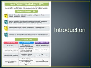
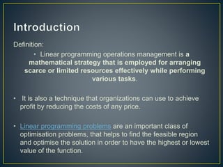
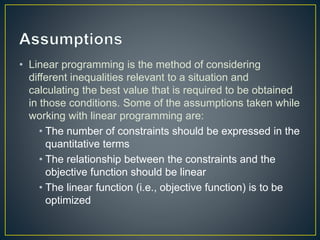
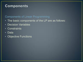
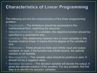
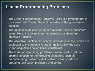
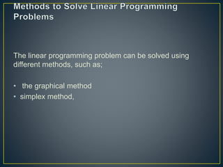
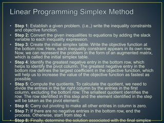
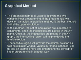
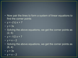
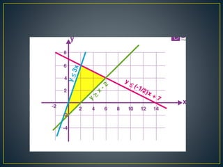
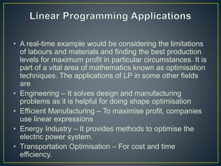
3. Definition:
• Linear programming operations management is a
mathematical strategy that is employed for arranging
scarce or limited resources effectively while performing
various tasks.
• It is also a technique that organizations can use to achieve
profit by reducing the costs of any price.
• Linear programming problems are an important class of
optimisation problems, that helps to find the feasible region
and optimise the solution in order to have the highest or lowest
value of the function.

4. • Linear programming is the method of considering
different inequalities relevant to a situation and
calculating the best value that is required to be obtained
in those conditions. Some of the assumptions taken while
working with linear programming are:
• The number of constraints should be expressed in the
quantitative terms
• The relationship between the constraints and the
objective function should be linear
• The linear function (i.e., objective function) is to be
optimized

5. Components of Linear Programming
• The basic components of the LP are as follows:
• Decision Variables
• Constraints
• Data
• Objective Functions

6. The following are the five characteristics of the linear programming
problem:
• Constraints – The limitations should be expressed in the
mathematical form, regarding the resource.
• Objective Function – In a problem, the objective function should be
specified in a quantitative way.
• Linearity – The relationship between two or more variables in the
function must be linear. It means that the degree of the variable is
one.
• Finiteness – There should be finite and infinite input and output
numbers. In case, if the function has infinite factors, the optimal
solution is not feasible.
• Non-negativity – The variable value should be positive or zero. It
should not be a negative value.
• Decision Variables – The decision variable will decide the output. It
gives the ultimate solution of the problem. For any problem, the first
step is to identify the decision variables.

7. • The Linear Programming Problems (LPP) is a problem that is
concerned with finding the optimal value of the given linear
function.
• The optimal value can be either maximum value or minimum
value. Here, the given linear function is considered an
objective function.
• The objective function can contain several variables, which are
subjected to the conditions and it has to satisfy the set of
linear inequalities called linear constraints.
• The linear programming problems can be used to get the
optimal solution for the following scenarios, such as
manufacturing problems, diet problems, transportation
problems, allocation problems and so on.

8. The linear programming problem can be solved using
different methods, such as;
• the graphical method
• simplex method,

9. • Step 1: Establish a given problem. (i.e.,) write the inequality constraints
and objective function.
• Step 2: Convert the given inequalities to equations by adding the slack
variable to each inequality expression.
• Step 3: Create the initial simplex table. Write the objective function at
the bottom row. Here, each inequality constraint appears in its own row.
Now, we can represent the problem in the form of an augmented matrix,
which is called the initial simplex table.
• Step 4: Identify the greatest negative entry in the bottom row, which
helps to identify the pivot column. The greatest negative entry in the
bottom row defines the largest coefficient in the objective function, which
will help us to increase the value of the objective function as fastest as
possible.
• Step 5: Compute the quotients. To calculate the quotient, we need to
divide the entries in the far right column by the entries in the first
column, excluding the bottom row. The smallest quotient identifies the
row. The row identified in this step and the element identified in the step
will be taken as the pivot element.
• Step 6: Carry out pivoting to make all other entries in column is zero.
• Step 7: If there are no negative entries in the bottom row, end the
process. Otherwise, start from step 4.
• Step 8: Finally, determine the solution associated with the final simplex

10. • The graphical method is used to optimize the two-
variable linear programming. If the problem has two
decision variables, a graphical method is the best method
to find the optimal solution.
• In this method, the set of inequalities are subjected to
constraints. Then the inequalities are plotted in the XY
plane. Once, all the inequalities are plotted in the XY
graph, the intersecting region will help to decide the
feasible region.
• The feasible region will provide the optimal solution as
well as explains what all values our model can take. Let
us see an example here and understand the concept of
linear programming in a better way.

11. Solution
The feasible region determined by the system of constraints, 3x+5y≤15,5x+2y≤10,x≥0,y≥0 are
as shown.
The corner points of the feasible region are O(0,0),A(2,0),B(0,3) and C(1920,1945)
The values of Z at these corner points are as follows.
Therefore, the maximum value of Z is 19235 at the point (1920,1945)

12. Corner
point
Z=5x+3y
O(0,0) 0
A(2,0) 10
B(0,3) 9
C(1920​,1945​)
19235​
→ Maximum

13. • Calculate the maximal and minimal value of z = 5x + 3y for the
following constraints.
• x + 2y ≤ 14
• 3x – y ≥ 0
• x – y ≤ 2
• Solution:
• The three inequalities indicate the constraints. The area of the
plane that will be marked is the feasible region.
• The optimisation equation (z) = 5x + 3y. You have to find the
(x,y) corner points that give the largest and smallest values of
z.
• To begin with, first solve each inequality.
• x + 2y ≤ 14 ⇒ y ≤ -(1/2)x + 7
• 3x – y ≥ 0 ⇒ y ≤ 3x
• x – y ≤ 2 ⇒ y ≥ x – 2

14. • Now pair the lines to form a system of linear equations to
find the corner points
• y = -(½) x + 7
• y = 3x
• Solving the above equations, we get the corner points as
(2, 6)
• y = -1/2 x + 7
• y = x – 2
• Solving the above equations, we get the corner points as
(6, 4)
• y = 3x
• y = x – 2

15. • Solving the above equations, we get the corner points as (-1, -
3)
• For linear systems, the maximum and minimum values of the
optimisation equation lie on the corners of the feasibility
region. Therefore, to find the optimum solution, you only need
to plug these three points in z = 3x + 4y
• (2, 6) :
• z = 5(2) + 3(6) = 10 + 18 = 28
• (6, 4):
• z = 5(6) + 3(4) = 30 + 12 = 42
• (–1, –3):
• z = 5(-1) + 3(-3) = -5 -9 = -14
• Hence, the maximum of z = 42 lies at (6, 4) and the minimum
of z = -14 lies at (-1, -3)

17. • A real-time example would be considering the limitations
of labours and materials and finding the best production
levels for maximum profit in particular circumstances. It is
part of a vital area of mathematics known as optimisation
techniques. The applications of LP in some other fields
are
• Engineering – It solves design and manufacturing
problems as it is helpful for doing shape optimisation
• Efficient Manufacturing – To maximise profit, companies
use linear expressions
• Energy Industry – It provides methods to optimise the
electric power system.
• Transportation Optimisation – For cost and time
efficiency.