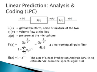
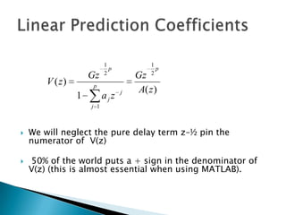
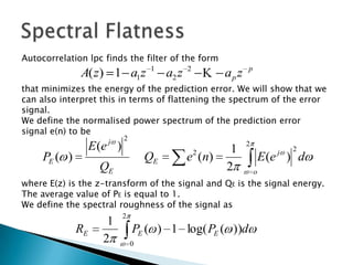
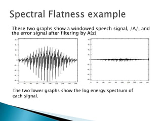
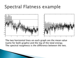
This document discusses linear prediction analysis (LPC) for speech recognition. It begins by deriving the linear prediction equations and describing the autocorrelation method of LPC. It then interprets the LPC filter as a spectral whitener that flattens the spectrum of the prediction error. The document discusses alternative methods like covariance LPC and closed phase covariance LPC. It also describes alternative parameter sets that can represent the LPC filter, such as pole positions, reflection coefficients, and log area ratios.

1. Methods and algorithms of speech recognition
course
Lection 4
Nikolay V. Karpov
nkarpov(а)hse.ru

2.  Aims of Linear Prediction
 Derivation of Linear Prediction Equations
 Autocorrelation method of LPC
 Interpretation of LPC filter as a spectral
whitener

3. u (n) = glottal waveform, noise or mixture of the two
ul (n ) = volume flow at the lips
s(n) = pressure at the microphone
1 1
p p
2 2
Gz Gz
V ( z) p
a time-varying all-pole filter
j A( z )
1 ajz
j 1
The aim of Linear Predication Analysis (LPC) is to
1
R( z ) 1 z
estimate V(z) from the speech signal s(n)

4. 1 1
p p
2 2
Gz Gz
V ( z) p
j A( z )
1 ajz
j 1
 We will neglect the pure delay term z–½ pin the
numerator of V(z)
 50% of the world puts a + sign in the denominator of
V(z) (this is almost essential when using MATLAB).

5. We can reverse the order of V(z) and R(z) since both are
linear and V(z) doesn’t change substantially during the
impulse response of R(z) or vice-versa
p
s(n) Gu' (n) a j s (n j)
j 1
If the vocal tract resonances have high gain, the second term will
dominate:

6. p
s(n) a j s(n j)
j 1
 The right hand side of this expression is a prediction of
s(n) as a linear sum of past speech samples. Define the
prediction error at sample n as
p
e( n ) s ( n) a j s(n j)
j 1
s (n) a1 (n 1) a2 (n 2) a p (n p)
or in terms of z-transform
E( z) S ( z ) A( z )

7. Given a frame of speech {F}, we would like to find the values ai
that minimize
QE e2 (n)
n {F }
To do so, we differentiate w.r.t each ai
QE e 2 (n) e(n)
2e(n) e(n)s(n i)
ai n {F } ai n {F } ai n {F }
The optimum values of ai must satisfy p equations
e(n)s(n i) 0; i 1 p
n {F }
p
e(n) s(n) a j s(n j)
j 1

8. p
s ( n) s ( n i ) a j s(n j ) s(n i) 0
n {F } j 1
p p
aj s (n j ) s (n i ) s ( n) s ( n i )
j 1 n {F } n {F }
p
ij aj i0 ; ij s (n i ) s (n j)
j 1 n {F }
or in matrix form
Φa c a Φ 1c
the matrix Φ is symmetric and positive semi-definite

9.  Symmetric ij ij ΦT Φ
 Positive for any x!=0
Definite xi ij x j 0 xT Φx 0
i, j
 Positive xi ij x j 0 xT Φx 0
Semi-
Definite: i, j
 Toeplitz: f (i j)
Constant i 1, j 1 ij
diagonals

10. Any special properties possessed by a matrix can
be used when inverting it to:
 reduce the computation time
 improve the accuracy
Matrix (pxp) Computation
General p3
Symmetric 1 3
p
2
Toeplitz, Symmetric,
+ve define
p2

11. We start with a frame of windowed speech
(typ 20-30 ms)
We take {F} to be infinite in extent ij s (n i) s(n j)
n
Because of the symmetry and the infinite sum, we have
ij i j ,0
Ri j
where the sequence Rk is the autocorrelation of the windowed speech.
The matrix Φ is now Toeplitz (has constant diagonals) and the
equations
Φa c
are called the Yule-Walker equations
Inverting a symmetric, positive definite, Toeplitz p×p matrix takes
O(p2) operations instead of the normal O(p3).
Inversion procedure is known as the
Levinson or Levinson-Durbin algorithm.

12. s ( n) E( z) S ( z ) A( z )
e( n )
Poles of V (z )

13. Autocorrelation lpc finds the filter of the form
1 2 p
A( z) 1 a1 z a2 z ap z
that minimizes the energy of the prediction error. We will show that we
can also interpret this in terms of flattening the spectrum of the error
signal.
We define the normalised power spectrum of the prediction error
signal e(n) to be
j 2
2
E (e ) 2 1 j 2
PE ( ) QE e (n) E (e ) d
QE 2 o
where E(z) is the z-transform of the signal and QE is the signal energy.
The average value of PE is equal to 1.
We define the spectral roughness of the signal as
2
1
RE PE ( ) 1 log( PE ( ))d
2 0

14. 2
1
RE PE ( ) 1 log( PE ( ))d
2 0
RE is similar to the variance of PE
since the integrand is similar to
1 2 where mean(PE)=1
( PE 1)
2
We can find an alternative expression for RE
2
1
RE log( PE ( ))d since PE ( )d 1
2 0
2 Thus the spectral roughness
1 2
of a signal equals the
log(QE ) - log E (e j ) d
2 0
difference between its log
energy and the average of
its log energy spectrum

15. We know that E( z) S ( z ) A( z )
j 2 j 2 j 2
log E (e ) log S (e ) log A(e )
Substituting this in the expression for RE gives
2 2
1 j 2 1 j 2
RE log(QE ) - log S (e ) d log A(e ) d
2 0
2 0
We saw in the section on filter properties that the term involving
A is zero since a0=1 and all roots of A lie in the unit circle. Hence
2
1 j 2
RE log(QE ) - log S (e ) d
2 0
The term involving S is independent of A. It follows that if A is
chosen to minimize QE, it will also minimize RE, the spectral
roughness of e(n). The filter A(z) is called a whitening filter
because it makes the spectrum flatter

16. These two graphs show a windowed speech signal, /A/, and
the error signal after filtering by A(z)
The two lower graphs show the log energy spectrum of
each signal.

17. The two horizontal lines on each graph are the mean value
(same for both graphs) and the log of the total energy.
The spectral roughness is the difference between the two.

18.  Covariance method of LPC
 Preemphasis
 Closed Phase Covariance LPC
 Alternative LPC parameter sets:
◦ Pole positions
◦ Reflection Coefficients
◦ Log Area Ratios

19.  We consider two variants of LPC analysis which differ
only in their choice of speech frame, {F}:
 Autocorrelation LPC Analysis
◦ Requires a windowed signal ⇒tradeoff between spectral
resolution and time resolution
◦ Requires >20 ms of data
◦ Has a fast algorithm because Φ is Toeplitz
◦ Guarantees a stable filter V(z)
 Covariance LPC Analysis (Prony’s method)
◦ No windowing required
◦ Gives infinite spectral resolution
◦ Requires >2 ms of data
◦ Slower algorithm because Φ is not Toeplitz
◦ Sometimes gives an unstable filter V(z)

20. From previous slide
p
ij aj i0 ; ij s (n i ) s (n j)
j 1 n {F }
We chose {F} to be a finite segment of speech: {F} = s(n) for
0 ≤ n ≤ (N-1) then we have:
ij s (n i ) s (n j)
n {F }
The matrix Φ is still symmetric but is no longer Toeplitz
N 2
ij s (n i 1) s (n j 1)
n 1
N 1
s( i)s( j ) s( N i)s( N j) s (n i 1) s (n j 1)
n 0
s( i)s( j ) s( N i)s( N j) i 1, j 1

21.  This allows the entire matrix Φ to be calculated
recursively from its first row or column.
 Since the matrix is not Toeplitz, the computation
involved in inverting Φ is ∝ p3 rather than ∝ p2
and so takes longer.
 Covariance LPC generally gives better results
than Autocorrelation LPC but is more sensitive to
the precise position of the frame in relation to
the vocal fold closures

22.  Covariance LPC does not necessarily give a stable filter
V(z)(though it usually does).
 We can force stability by replacing an unstable pole at z= p by a
stable one at z= 1/p*
As we have seen in the section on filter properties, reflecting a pole in
the unit circle leaves the magnitude response unchanged except for
multiplying by a constant (equal to the magnitude of the pole).
Thus the spectral flattening property of LPC is unaltered by
this pole reflection.
Discovering which poles lie outside the unit circle is quite expensive:
this is a further computational disadvantage of covariance LPC

23.  The matrix Φ is always non-singular, but not necessarily by very much. A
measure of how close a matrix is to being singular is given by its
condition number: for a symmetric +ve definite matrix, this is the ratio
of its largest to its smallest eigenvalue.
 For large p, the condition number of Φ tends to the ratio
Smax(ω)/Smin(ω). We can thus improve the numerical properties of the
LPC analysis procedure by flattening the speech spectrum before
calculating the autocorrelation matrix Φ.
 For voiced speech, the input to V(z) is ug′(n) whose spectrum falls off at
high frequencies at around – 6dB/octave. This can be compensated with
a 1st-order high-pass filter with a zero near z=1: 1
P( z ) 1 z
 P(z) is approximately a differentiator. The normalised corner frequency
of P(z)is approximately (1–α)/2π: This is typically placed in the range 0
to 150 Hz. From a spectral flatness point of view, the optimum value of
αis φ10/φ00 (obtained from autocorrelation LPC with p= 1)

24. p
From previous slide s(n) Gu' (n) a j s (n j)
j 1
We have neglected the term Gu′(n) because we don’t know
what it is and it is assumed to be much smaller than the
second term.
If we knew when the vocal folds were closed, we could
restrict {F} to those particular intervals. We can estimate the
times of vocal fold closure in two ways:
 Looking for spikes in the e(n) signal
 Using a Laryngograph (or Electroglottograph or EGG): this
instrument measures the radio-frequency conductance
across the larynx.
◦ Conductance ∝Vocal fold contact area.
◦ Accurate but inconvenient.
In Closed-Phase LPC, we choose our analysis interval {F} to
consist of one or more closed phase intervals (not
necessarily contiguous). No preemphasis is necessary
because the excitation now has a flat spectrum.

25. s(n)
V (e j T )
e(n) ug ' (n)
u g (n)
Frequency (Hz)

26. The vocal tract filter is defined by p+1parameters:
G
V ( z) p
j
1 ajz
j 1
The LPC (or AR) coefficients a have some bad properties:
 The frequency response is very sensitive to small changes
in a (such as quantizing errors in coding)
 There is no easy way to verify that the filter is stable
 Interpolating between the parameters that correspond to
two different filters will not vary the frequency response
smoothly from one to the other: stability is not even
guaranteed.
 There are several alternative parameter sets that are
equivalent to the a (most require G to be specified as well)

27. We can factorize the denominator of V(z) to give its poles
p p
j
1 ajz (1 xk z 1 )
j 1 k 1
 The polynomial roots xk are either real or occur in
complex conjugate pairs. |xk| must be <1 for stability.
Factorizing polynomials is computationally expensive.
The frequency response is sensitive to pole position
errors near |z|=1

28.  Any all-pole filter is equivalent to a tube with p sections:
this is characterised by p reflection coefficients (assuming
r0=1). We can convert between the reflection coefficients
and the polynomial coefficients by using the formulae given
previously.
Properties:
 An all-pole filter is stable if the corresponding reflection
coefficients all lie between -1 and +1.
 Interpolating between two of reflection coefficient sets will
give a smoothly changing frequency response.
 High coefficient sensitivity near ±1.
 The negative reflection coefficients are sometimes called
the PARCOR coefficients (PARCOR = partial correlation).

29. Ai 1 1 ri e gi 1 gi
gi log log ri tanh( )
Ai 1 ri e gi 1 2
Stability is guaranteed for any values of gi.
Reflection
coefficient
Log-Area Coefficient