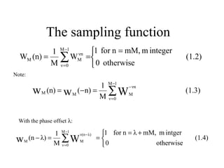
Download to read offline


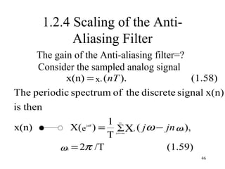
![−λ
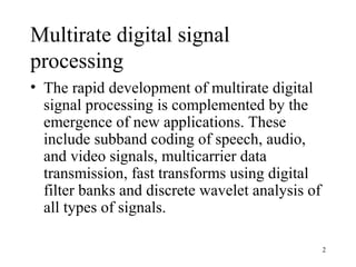
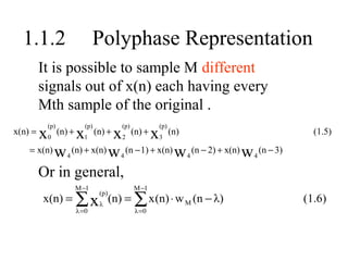
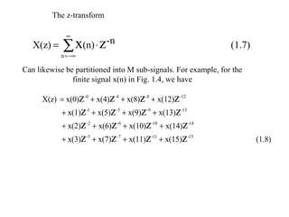
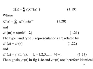
Taking out factor of z , λ = 0.....3, gives
[
-0 -0 -4 -8
x( z ) = z x(0) z + x(4) z + x(8) z + x(12) z ] -12
+ z [ x(1) z + x(5) z + x(9) z + x(13) z ]
-1 -0 -4 -8 -12
+ z [ x(2) z + x(6) z + x(10) z + x(14) z ]
-2 -0 -4 -8 -12
+ z [ x(3) z + x(7) z + x(11) z + x(15) z ]
-3 -0 -4 -8 -12
(1.9)
These are polynomials in z-4
12](https://image.slidesharecdn.com/dsp3-120829141828-phpapp02/85/Dsp3-12-320.jpg)
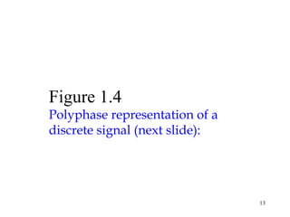
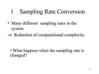
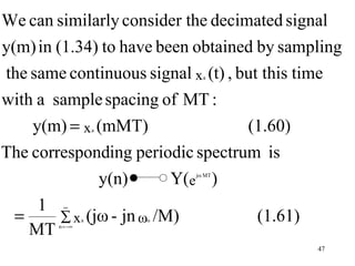
![First polynomial :
(p) −0 −1 −2 −3
x 0
( z ) = x(0) z + x(4) z + x(8) z + x(12) z (1.12)
One-to-one Mapping
z n
-λ ( p) M ( p)
z xλ ( z ) xλ (n), λ = 0,1,2.... M - 1 (1.13)
Vector Form :
X
(p)
(z) = [X (p)
0
(z), z
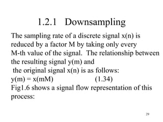
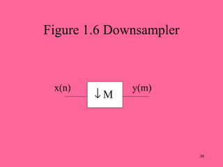
−1
X
1
(p)
(z),...., z
− (M −1)
X
(p)
M −1
(z) ]
T
(1.14)
16](https://image.slidesharecdn.com/dsp3-120829141828-phpapp02/85/Dsp3-16-320.jpg)
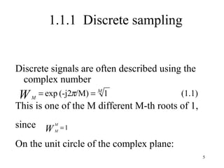
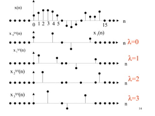
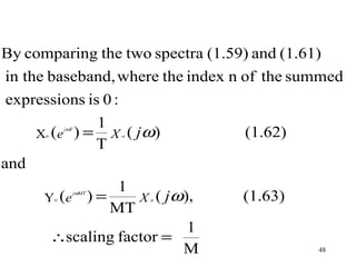
![Replacing λ by M - 1 - λ leads to the type 2 polyphase representation
[ Vai 88b] :
M −1
X(z) = ∑ z
− (m −1− λ) (p2) M
λ =0
X λ
(z ) (1.15)
Where
∞
∑x
(p2) M (p2) − mM
X (z λ
)=
m =-∞
λ
(m). z (1.16)
and
(p2)
x λ
(m) = x(mM + M − 1 − λ) (1.17)
17](https://image.slidesharecdn.com/dsp3-120829141828-phpapp02/85/Dsp3-17-320.jpg)
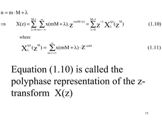
![The type 1 and type 2 representations are related by
(z) = x M −1− λ (z),
(p2) (p)
x λ
λ = 0,1,2........ M - 1 (1.18)
(p) (p2)
The signals x1 (n) from Fig.1.4c and x 2 (n)
are therefore identical. Only the indexing is done
in the reverse order.
Replacing λ by - λ the type 3 polyphase
representation will be obtained
from the standard representation [ Cro 83] :
18](https://image.slidesharecdn.com/dsp3-120829141828-phpapp02/85/Dsp3-18-320.jpg)
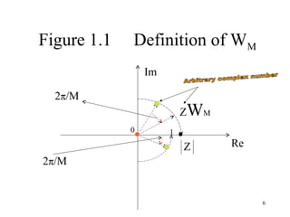
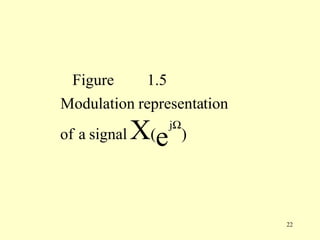
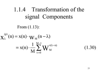
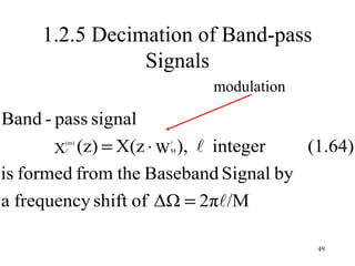
![1.1.3 Modulation Representation
Multiply the argument z by W k
M
(m)
X (e
k
X(z W ), k = 0,1,2....M -1
jΩ
)=
k
M
(1.24)
jΩ
Z → e ( Fourier Transform)
X (e ) = X(e e ) = X(e
(m) jΩ jΩ - j2π k/M j[ Ω - 2π k/M]
) (1.25)
k
2π k
Modulation = shifting the frequency by
M
20](https://image.slidesharecdn.com/dsp3-120829141828-phpapp02/85/Dsp3-20-320.jpg)
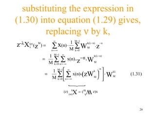
![To avoid complex Time Domain signals
we have to combine
X(z W k
M
) + X(z W M )
M -k
W
- kn
M
kn
x(n) + W M x(n)
= 2x(n) ⋅ cos(2π kn/M) (1.27)
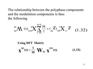
The complete set of modulated z - Transforms
in the Matrix form :
x
(m)
(z) = [x (m)
0
(z) x 1
(m)
(z) ...... x
(m)
M −1
(z) ] T
(1.28)
∞
∑X
-λ (p) M (p) −n
z X λ
(z ) =
m = −∞
λ
.z (1.29)
24](https://image.slidesharecdn.com/dsp3-120829141828-phpapp02/85/Dsp3-24-320.jpg)
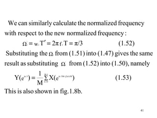
![Normalised Sampling Rate is 2π
Magnitude is decreased by factor M
2π
New sampling rate
M
⇒ s = jω
e =e =e =e (1.48)
jMΩ jMω T jωT ′ jΩ ′
The normalized frequency Ω′ = MΩ (1.49)
corresponds time spacing T′
Spectrum in terms of Ω′
1
⇒ Y(e ) = ∑ X(e
M −1
j Ω′ j[ Ω′− 2π k]/M
) (1.50)
M k =0
39](https://image.slidesharecdn.com/dsp3-120829141828-phpapp02/85/Dsp3-39-320.jpg)
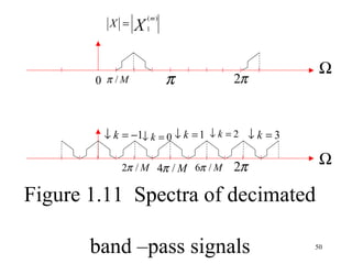
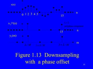
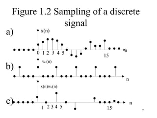
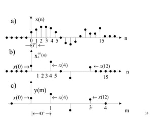
![fig 1.13a shows the signal x(n), already given
in the fig 1.2a, and fig 1.13b the polyphase
components x (n). From here, we can obtain
(p)
2
the downsampled signal y (m) shown 2
in fig. 1.13c, by replacing z by Z or M
Ω by Ω / M , respectively (see section 1.2.1).
Its spectrum is therefore
y (m)
λ Y (e ) λ
jΩ
= 1 ∑ X(e j[ Ω−2 πk ] / M ) ⋅ W kλ
M −1
M k =0 M (1.71)
57](https://image.slidesharecdn.com/dsp3-120829141828-phpapp02/85/Dsp3-57-320.jpg)
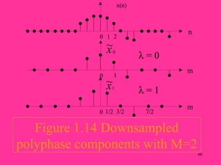
![Fig 1.14b shows the downsampled component ~ (m), (p)
0 x
i.e. for λ = 0 . Substituti ng M = 2 into (1.70), we obtain
the spectrum :
~
11
x
(p)
0 ∑ X(e ) j[Ω −πk]
(1.72)
2
k =0
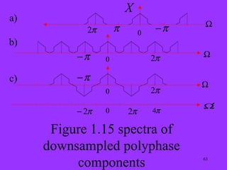
This spectrum is shown in fig 1.15b. The two sum terms
combine to form a real spectrum with a period Ω = π
or Ω′ = 2ππrespctivly. This result is seen to be compatible
with having a phase offest λ = 0 and having reduced the
sampling rate by afactor of 2 (see section 1.2.2).
~ 1 1
x
(p)
1 ∑ X(e ) W ,
j[Ω −πk]
(1.73)
K
2
2k =0
( −1)
k
61](https://image.slidesharecdn.com/dsp3-120829141828-phpapp02/85/Dsp3-61-320.jpg)


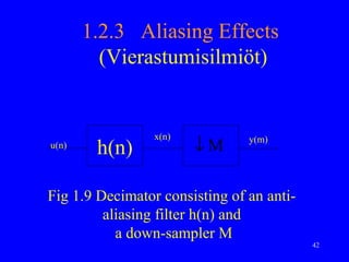
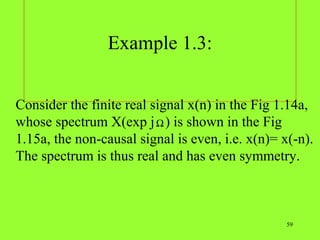
The document provides information about Expert Systems and Solutions, including their contact details and areas of expertise. They are calling for research projects from final year students in fields like electrical engineering, electronics and communications, power systems, and applied electronics. Students can assemble hardware projects in the company's research labs with guidance from experts.


![Getting Started with Apache Spark: Big Data Made Simple [Free Meetup]](https://cdn.slidesharecdn.com/ss_thumbnails/apachesparkgettingstarted-260203175547-8361bcc3-thumbnail.jpg?width=640&height=640&fit=bounds)


