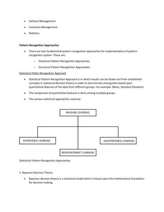
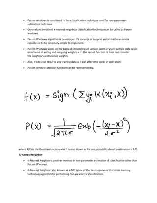
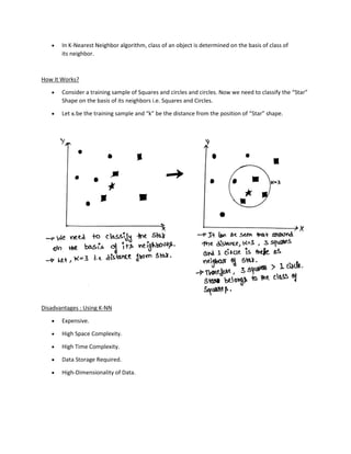
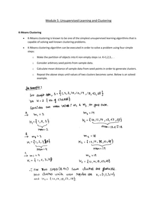
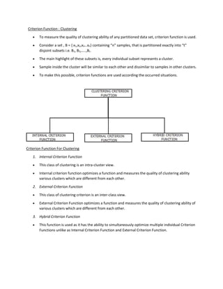
Bayesian classification is a statistical classification method that uses Bayes' theorem to calculate the probability of class membership. It provides probabilistic predictions by calculating the probabilities of classes for new data based on training data. The naive Bayesian classifier is a simple Bayesian model that assumes conditional independence between attributes, allowing faster computation. Bayesian belief networks are graphical models that represent dependencies between variables using a directed acyclic graph and conditional probability tables.
Machine Learning and Real-World ApplicationsMachinePulse
This presentation was created by Ajay, Machine Learning Scientist at MachinePulse, to present at a Meetup on Jan. 30, 2015. These slides provide an overview of widely used machine learning algorithms. The slides conclude with examples of real world applications.
Ajay Ramaseshan, is a Machine Learning Scientist at MachinePulse. He holds a Bachelors degree in Computer Science from NITK, Suratkhal and a Master in Machine Learning and Data Mining from Aalto University School of Science, Finland. He has extensive experience in the machine learning domain and has dealt with various real world problems.
The document discusses pattern recognition including defining a pattern and pattern class, examples of pattern recognition applications, and the statistical and machine learning approaches used. It provides details on the human and machine perception of patterns and the typical pattern recognition process of data acquisition, preprocessing, feature extraction, classification, and post processing. It also presents a case study on using pattern recognition for fish classification to sort sea bass and salmon.
This document provides an overview of pattern recognition techniques. It begins with an introduction to pattern recognition and its applications. It then outlines the syllabus, which includes topics like design principles, statistical pattern recognition, parameter estimation methods, principal component analysis, linear discriminant analysis, and classification techniques. Under each topic, it provides further details and explanations.
This document discusses rule-based classification. It describes how rule-based classification models use if-then rules to classify data. It covers extracting rules from decision trees and directly from training data. Key points include using sequential covering algorithms to iteratively learn rules that each cover positive examples of a class, and measuring rule quality based on both coverage and accuracy to determine the best rules.
The document discusses various model-based clustering techniques for handling high-dimensional data, including expectation-maximization, conceptual clustering using COBWEB, self-organizing maps, subspace clustering with CLIQUE and PROCLUS, and frequent pattern-based clustering. It provides details on the methodology and assumptions of each technique.
The document discusses the K-nearest neighbors (KNN) algorithm, a simple machine learning algorithm used for classification problems. KNN works by finding the K training examples that are closest in distance to a new data point, and assigning the most common class among those K examples as the prediction for the new data point. The document covers how KNN calculates distances between data points, how to choose the K value, techniques for handling different data types, and the strengths and weaknesses of the KNN algorithm.
The document summarizes statistical pattern recognition techniques. It is divided into 9 sections that cover topics like dimensionality reduction, classifiers, classifier combination, and unsupervised classification. The goal of pattern recognition is supervised or unsupervised classification of patterns based on features. Dimensionality reduction aims to reduce the number of features to address the curse of dimensionality when samples are limited. Multiple classifiers can be combined through techniques like stacking, bagging, and boosting. Unsupervised classification uses clustering algorithms to construct decision boundaries without labeled training data.
The document discusses different approaches for concept learning from examples, including viewing it as a search problem to find the hypothesis that best fits the training examples. It also describes the general-to-specific learning approach, where the goal is to find the maximally specific hypothesis consistent with the positive training examples by starting with the most general hypothesis and replacing constraints to better fit the examples. The document also discusses the version space and candidate elimination algorithms for obtaining the version space of all hypotheses consistent with the training data.
A short presentation for beginners on Introduction of Machine Learning, What it is, how it works, what all are the popular Machine Learning techniques and learning models (supervised, unsupervised, semi-supervised, reinforcement learning) and how they works with various Industry use-cases and popular examples.
The document discusses bagging, an ensemble machine learning method. Bagging (bootstrap aggregating) uses multiple models fitted on random subsets of a dataset to improve stability and accuracy compared to a single model. It works by training base models in parallel on random samples with replacement of the original dataset and aggregating their predictions. Key benefits are reduced variance, easier implementation through libraries like scikit-learn, and improved performance over single models. However, bagging results in less interpretable models compared to a single model.
This document discusses Bayesian learning and the Bayes theorem. Some key points:
- Bayesian learning uses probabilities to calculate the likelihood of hypotheses given observed data and prior probabilities. The naive Bayes classifier is an example.
- The Bayes theorem provides a way to calculate the posterior probability of a hypothesis given observed training data by considering the prior probability and likelihood of the data under the hypothesis.
- Bayesian methods can incorporate prior knowledge and probabilistic predictions, and classify new instances by combining predictions from multiple hypotheses weighted by their probabilities.
Convolutional neural networks (CNNs) learn multi-level features and perform classification jointly and better than traditional approaches for image classification and segmentation problems. CNNs have four main components: convolution, nonlinearity, pooling, and fully connected layers. Convolution extracts features from the input image using filters. Nonlinearity introduces nonlinearity. Pooling reduces dimensionality while retaining important information. The fully connected layer uses high-level features for classification. CNNs are trained end-to-end using backpropagation to minimize output errors by updating weights.
Decision tree is a type of supervised learning algorithm (having a pre-defined target variable) that is mostly used in classification problems. It is a tree in which each branch node represents a choice between a number of alternatives, and each leaf node represents a decision.
This presentation introduces naive Bayesian classification. It begins with an overview of Bayes' theorem and defines a naive Bayes classifier as one that assumes conditional independence between predictor variables given the class. The document provides examples of text classification using naive Bayes and discusses its advantages of simplicity and accuracy, as well as its limitation of assuming independence. It concludes that naive Bayes is a commonly used and effective classification technique.
This document provides an overview of pattern classification and clustering algorithms. It defines key concepts like pattern recognition, supervised and unsupervised learning. For pattern classification, it discusses algorithms like decision trees, kernel estimation, K-nearest neighbors, linear discriminant analysis, quadratic discriminant analysis, naive Bayes classifier and artificial neural networks. It provides examples to illustrate decision tree classification and information gain calculation. For clustering, it mentions hierarchical, K-means and KPCA clustering algorithms. The document is a guide to pattern recognition models and algorithms for classification and clustering.
BIRCH (balanced iterative reducing and clustering using hierarchies) is an unsupervised data-mining algorithm used to perform hierarchical clustering over, particularly large data sets.
This document discusses inductive bias in machine learning. It defines inductive bias as the assumptions that allow an inductive learning system to generalize beyond its training data. Without some biases, a learning system cannot rationally classify new examples. The document compares different learning algorithms based on the strength of their inductive biases, from weak biases like rote learning to stronger biases like preferring more specific hypotheses. It argues that all inductive learning systems require some inductive biases to generalize at all.
This document discusses and provides examples of supervised and unsupervised learning. Supervised learning involves using labeled training data to learn relationships between inputs and outputs and make predictions. An example is using data on patients' attributes to predict the likelihood of a heart attack. Unsupervised learning involves discovering hidden patterns in unlabeled data by grouping or clustering items with similar attributes, like grouping fruits by color without labels. The goal of supervised learning is to build models that can make predictions when new examples are presented.
This presentation was prepared as part of the curriculum studies for CSCI-659 Topics in Artificial Intelligence Course - Machine Learning in Computational Linguistics.
It was prepared under guidance of Prof. Sandra Kubler.
Introdution and designing a learning systemswapnac12
The document discusses machine learning and provides definitions and examples. It covers the following key points:
- Machine learning is a subfield of artificial intelligence concerned with developing algorithms that allow computers to learn from data without being explicitly programmed.
- Well-posed learning problems have a defined task, performance measure, and training experience. Examples given include learning to play checkers and recognize handwritten words.
- Designing a machine learning system involves choosing a training experience, target function, representation of the target function, and learning algorithm to approximate the function. A checkers-playing example is used to illustrate these design decisions.
Ensemble Learning is a technique that creates multiple models and then combines them to produce improved results.
Ensemble learning usually produces more accurate solutions than a single model would.
The document is a chapter from a textbook on data mining written by Akannsha A. Totewar, a professor at YCCE in Nagpur, India. It provides an introduction to data mining, including definitions of data mining, the motivation and evolution of the field, common data mining tasks, and major issues in data mining such as methodology, performance, and privacy.
Outlier analysis is used to identify outliers, which are data objects that are inconsistent with the general behavior or model of the data. There are two main types of outlier detection - statistical distribution-based detection, which identifies outliers based on how far they are from the average statistical distribution, and distance-based detection, which finds outliers based on how far they are from other data objects. Outlier analysis is useful for tasks like fraud detection, where outliers may indicate fraudulent activity that is different from normal patterns in the data.
This document provides an overview of PAC (Probably Approximately Correct) learning theory. It discusses how PAC learning relates the probability of successful learning to the number of training examples, complexity of the hypothesis space, and accuracy of approximating the target function. Key concepts explained include training error vs true error, overfitting, the VC dimension as a measure of hypothesis space complexity, and how PAC learning bounds can be derived for finite and infinite hypothesis spaces based on factors like the training size and VC dimension.
Scikit-Learn is a powerful machine learning library implemented in Python with numeric and scientific computing powerhouses Numpy, Scipy, and matplotlib for extremely fast analysis of small to medium sized data sets. It is open source, commercially usable and contains many modern machine learning algorithms for classification, regression, clustering, feature extraction, and optimization. For this reason Scikit-Learn is often the first tool in a Data Scientists toolkit for machine learning of incoming data sets.
The purpose of this one day course is to serve as an introduction to Machine Learning with Scikit-Learn. We will explore several clustering, classification, and regression algorithms for a variety of machine learning tasks and learn how to implement these tasks with our data using Scikit-Learn and Python. In particular, we will structure our machine learning models as though we were producing a data product, an actionable model that can be used in larger programs or algorithms; rather than as simply a research or investigation methodology.
Pattern Recognition is the branch of machine learning a computer science which deals with the regularities and patterns in the data that can further be used to classify and categorize the data with the help of Pattern Recognition System.
“The assignment of a physical object or event to one of several pre-specified categories”-- Duda & Hart
Pattern Recognition System is responsible for generating patterns and similarities among given problem/data space, that can further be used to generate solutions to complex problems effectively and efficiently.
Certain problems that can be solved by humans, can also be made to be solved by machine by using this process.
UNIT 3: Data Warehousing and Data MiningNandakumar P
UNIT-III Classification and Prediction: Issues Regarding Classification and Prediction – Classification by Decision Tree Introduction – Bayesian Classification – Rule Based Classification – Classification by Back propagation – Support Vector Machines – Associative Classification – Lazy Learners – Other Classification Methods – Prediction – Accuracy and Error Measures – Evaluating the Accuracy of a Classifier or Predictor – Ensemble Methods – Model Section.
Data mining involves finding hidden patterns in large datasets. It differs from traditional data access in that the query may be unclear, the data has been preprocessed, and the output is an analysis rather than a data subset. Data mining algorithms attempt to fit models to the data by examining attributes, criteria for preference of one model over others, and search techniques. Common data mining tasks include classification, regression, clustering, association rule learning, and prediction.
Statistical theory is a branch of mathematics and statistics that provides the foundation for understanding and working with data, making inferences, and drawing conclusions from observed phenomena. It encompasses a wide range of concepts, principles, and techniques for analyzing and interpreting data in a systematic and rigorous manner. Statistical theory is fundamental to various fields, including science, social science, economics, engineering, and more.
The document discusses the differences and similarities between classification and prediction, providing examples of how classification predicts categorical class labels by constructing a model based on training data, while prediction models continuous values to predict unknown values, though the process is similar between the two. It also covers clustering analysis, explaining that it is an unsupervised technique that groups similar data objects into clusters to discover hidden patterns in datasets.
This document analyzes and compares different statistical and machine learning methods for software effort prediction, including linear regression, support vector machine, artificial neural network, decision tree, and bagging. The researchers tested these methods on a dataset of 499 software projects. Their results showed that the decision tree method produced more accurate effort predictions than the other methods tested, performing comparably to linear regression. The decision tree approach is therefore considered effective for software effort estimation.
This document discusses various techniques for data classification including decision tree induction, Bayesian classification methods, rule-based classification, and classification by backpropagation. It covers key concepts such as supervised vs. unsupervised learning, training data vs. test data, and issues around preprocessing data for classification. The document also discusses evaluating classification models using metrics like accuracy, precision, recall, and F-measures as well as techniques like holdout validation, cross-validation, and bootstrap.
Machine learning is a type of artificial intelligence that allows software to learn from data without being explicitly programmed. The document discusses several machine learning techniques including supervised learning algorithms like linear regression, logistic regression, decision trees, support vector machines, K-nearest neighbors, and Naive Bayes. Unsupervised learning algorithms covered include clustering techniques like K-means and hierarchical clustering. Applications of machine learning include spam filtering, fraud detection, image recognition, and medical diagnosis.
This document discusses various types of machine learning. It begins by defining learning as changes that enable a system to perform tasks more efficiently over time through constructing or modifying representations of experiences. It then covers several types of learning including rote learning, learning by taking advice, learning through problem solving via parameter adjustment and chunking, learning from examples through induction, explanation based learning, learning through discovery and analogy. It also discusses formal learning theory and neural network and genetic learning. Key aspects of learning systems and different learning paradigms are described.
The document discusses different approaches to artificial intelligence, including rule-based and learning-based systems. It describes rule-based systems as using if-then rules to reach conclusions, while learning-based systems can adapt existing knowledge through learning. Machine learning is discussed as a type of learning-based AI that allows systems to learn from data without being explicitly programmed. Deep learning is described as a subset of machine learning that uses neural networks with multiple layers to learn from examples in a way similar to the human brain.
Classification models are used to categorize data into discrete classes or categories. For example, classifying loan applications as "safe" or "risky". The classification process involves building a classifier or model from training data using a classification algorithm, then applying the classifier to new data to categorize it. Prediction models are used to predict continuous numeric values, like estimating how much a customer will spend on a computer based on their income and occupation. The main difference is that classification predicts discrete classes while prediction estimates numeric values.
Identifying and classifying unknown Network Disruptionjagan477830
This document discusses identifying and classifying unknown network disruptions using machine learning algorithms. It begins by introducing the problem and importance of identifying network disruptions. Then it discusses related work on classifying network protocols. The document outlines the dataset and problem statement of predicting fault severity. It describes the machine learning workflow and various algorithms like random forest, decision tree and gradient boosting that are evaluated on the dataset. Finally, it concludes with achieving the objective of classifying disruptions and discusses future work like optimizing features and using neural networks.
This document discusses classification and prediction techniques for data analysis. Classification predicts categorical labels, while prediction models continuous values. Common algorithms include decision tree induction and Naive Bayesian classification. Decision trees use measures like information gain to build classifiers by recursively partitioning training data. Naive Bayesian classifiers apply Bayes' theorem to estimate probabilities for classification. Both approaches are popular due to their accuracy, speed and interpretability.
This slide gives brief overview of supervised, unsupervised and reinforcement learning. Algorithms discussed are Naive Bayes, K nearest neighbour, SVM,decision tree, Markov model.
Difference between regression and classification. difference between supervised and reinforcement, iterative functioning of Markov model and machine learning applications.
Classification is a popular data mining technique that assigns items to target categories or classes. It builds models called classifiers to predict the class of records with unknown class labels. Some common applications of classification include fraud detection, target marketing, and medical diagnosis. Classification involves a learning step where a model is constructed by analyzing a training set with class labels, and a classification step where the model predicts labels for new data. Supervised learning uses labeled data to train machine learning algorithms to produce correct outcomes for new examples.
This document provides an introduction to machine learning for data science. It discusses the applications and foundations of data science, including statistics, linear algebra, computer science, and programming. It then describes machine learning, including the three main categories of supervised learning, unsupervised learning, and reinforcement learning. Supervised learning algorithms covered include logistic regression, decision trees, random forests, k-nearest neighbors, and support vector machines. Unsupervised learning methods discussed are principal component analysis and cluster analysis.
In a world of data explosion, the rate of data generation and consumption is on the increasing side,
there comes the buzzword - Big Data.
Big Data is the concept of fast-moving, large-volume data in varying dimensions (sources) and
highly unpredicted sources.
The 4Vs of Big Data
● Volume - Scale of Data
● Velocity - Analysis of Streaming Data
● Variety - Different forms of Data
● Veracity - Uncertainty of Data
With increasing data availability, the new trend in the industry demands not just data collection but making an ample sense of acquired data - thereby, the concept of Data Analytics.
Taking it a step further to further make futuristic prediction and realistic inferences - the concept
of Machine Learning.
A blend of both gives a robust analysis of data for the past, now and the future.
There is a thin line between data analytics and Machine learning which becomes very obvious
when you dig deep.
1. Singular Value Decomposition (SVD) is a matrix factorization technique that decomposes a matrix into three other matrices.
2. SVD is primarily used for dimensionality reduction, information extraction, and noise reduction.
3. Key applications of SVD include matrix approximation, principal component analysis, image compression, recommendation systems, and signal processing.
EDAB Module 5 Singular Value Decomposition (SVD).pptxrajalakshmi5921
1. Singular Value Decomposition (SVD) is a matrix factorization technique that decomposes a matrix into three other matrices.
2. SVD is primarily used for dimensionality reduction, information extraction, and noise reduction.
3. Key applications of SVD include matrix approximation, principal component analysis, image compression, recommendation systems, and signal processing.
Gas agency management system project report.pdfKamal Acharya
The project entitled "Gas Agency" is done to make the manual process easier by making it a computerized system for billing and maintaining stock. The Gas Agencies get the order request through phone calls or by personal from their customers and deliver the gas cylinders to their address based on their demand and previous delivery date. This process is made computerized and the customer's name, address and stock details are stored in a database. Based on this the billing for a customer is made simple and easier, since a customer order for gas can be accepted only after completing a certain period from the previous delivery. This can be calculated and billed easily through this. There are two types of delivery like domestic purpose use delivery and commercial purpose use delivery. The bill rate and capacity differs for both. This can be easily maintained and charged accordingly.
Digital Twins Computer Networking Paper Presentation.pptxaryanpankaj78
A Digital Twin in computer networking is a virtual representation of a physical network, used to simulate, analyze, and optimize network performance and reliability. It leverages real-time data to enhance network management, predict issues, and improve decision-making processes.
Comparative analysis between traditional aquaponics and reconstructed aquapon...bijceesjournal
The aquaponic system of planting is a method that does not require soil usage. It is a method that only needs water, fish, lava rocks (a substitute for soil), and plants. Aquaponic systems are sustainable and environmentally friendly. Its use not only helps to plant in small spaces but also helps reduce artificial chemical use and minimizes excess water use, as aquaponics consumes 90% less water than soil-based gardening. The study applied a descriptive and experimental design to assess and compare conventional and reconstructed aquaponic methods for reproducing tomatoes. The researchers created an observation checklist to determine the significant factors of the study. The study aims to determine the significant difference between traditional aquaponics and reconstructed aquaponics systems propagating tomatoes in terms of height, weight, girth, and number of fruits. The reconstructed aquaponics system’s higher growth yield results in a much more nourished crop than the traditional aquaponics system. It is superior in its number of fruits, height, weight, and girth measurement. Moreover, the reconstructed aquaponics system is proven to eliminate all the hindrances present in the traditional aquaponics system, which are overcrowding of fish, algae growth, pest problems, contaminated water, and dead fish.
Build the Next Generation of Apps with the Einstein 1 Platform.
Rejoignez Philippe Ozil pour une session de workshops qui vous guidera à travers les détails de la plateforme Einstein 1, l'importance des données pour la création d'applications d'intelligence artificielle et les différents outils et technologies que Salesforce propose pour vous apporter tous les bénéfices de l'IA.
Introduction- e - waste – definition - sources of e-waste– hazardous substances in e-waste - effects of e-waste on environment and human health- need for e-waste management– e-waste handling rules - waste minimization techniques for managing e-waste – recycling of e-waste - disposal treatment methods of e- waste – mechanism of extraction of precious metal from leaching solution-global Scenario of E-waste – E-waste in India- case studies.
Rainfall intensity duration frequency curve statistical analysis and modeling...bijceesjournal
Using data from 41 years in Patna’ India’ the study’s goal is to analyze the trends of how often it rains on a weekly, seasonal, and annual basis (1981−2020). First, utilizing the intensity-duration-frequency (IDF) curve and the relationship by statistically analyzing rainfall’ the historical rainfall data set for Patna’ India’ during a 41 year period (1981−2020), was evaluated for its quality. Changes in the hydrologic cycle as a result of increased greenhouse gas emissions are expected to induce variations in the intensity, length, and frequency of precipitation events. One strategy to lessen vulnerability is to quantify probable changes and adapt to them. Techniques such as log-normal, normal, and Gumbel are used (EV-I). Distributions were created with durations of 1, 2, 3, 6, and 24 h and return times of 2, 5, 10, 25, and 100 years. There were also mathematical correlations discovered between rainfall and recurrence interval.
Findings: Based on findings, the Gumbel approach produced the highest intensity values, whereas the other approaches produced values that were close to each other. The data indicates that 461.9 mm of rain fell during the monsoon season’s 301st week. However, it was found that the 29th week had the greatest average rainfall, 92.6 mm. With 952.6 mm on average, the monsoon season saw the highest rainfall. Calculations revealed that the yearly rainfall averaged 1171.1 mm. Using Weibull’s method, the study was subsequently expanded to examine rainfall distribution at different recurrence intervals of 2, 5, 10, and 25 years. Rainfall and recurrence interval mathematical correlations were also developed. Further regression analysis revealed that short wave irrigation, wind direction, wind speed, pressure, relative humidity, and temperature all had a substantial influence on rainfall.
Originality and value: The results of the rainfall IDF curves can provide useful information to policymakers in making appropriate decisions in managing and minimizing floods in the study area.
Embedded machine learning-based road conditions and driving behavior monitoringIJECEIAES
Car accident rates have increased in recent years, resulting in losses in human lives, properties, and other financial costs. An embedded machine learning-based system is developed to address this critical issue. The system can monitor road conditions, detect driving patterns, and identify aggressive driving behaviors. The system is based on neural networks trained on a comprehensive dataset of driving events, driving styles, and road conditions. The system effectively detects potential risks and helps mitigate the frequency and impact of accidents. The primary goal is to ensure the safety of drivers and vehicles. Collecting data involved gathering information on three key road events: normal street and normal drive, speed bumps, circular yellow speed bumps, and three aggressive driving actions: sudden start, sudden stop, and sudden entry. The gathered data is processed and analyzed using a machine learning system designed for limited power and memory devices. The developed system resulted in 91.9% accuracy, 93.6% precision, and 92% recall. The achieved inference time on an Arduino Nano 33 BLE Sense with a 32-bit CPU running at 64 MHz is 34 ms and requires 2.6 kB peak RAM and 139.9 kB program flash memory, making it suitable for resource-constrained embedded systems.
Software Engineering and Project Management - Software Testing + Agile Method...Prakhyath Rai
Software Testing: A Strategic Approach to Software Testing, Strategic Issues, Test Strategies for Conventional Software, Test Strategies for Object -Oriented Software, Validation Testing, System Testing, The Art of Debugging.
Agile Methodology: Before Agile – Waterfall, Agile Development.
Discover the latest insights on Data Driven Maintenance with our comprehensive webinar presentation. Learn about traditional maintenance challenges, the right approach to utilizing data, and the benefits of adopting a Data Driven Maintenance strategy. Explore real-world examples, industry best practices, and innovative solutions like FMECA and the D3M model. This presentation, led by expert Jules Oudmans, is essential for asset owners looking to optimize their maintenance processes and leverage digital technologies for improved efficiency and performance. Download now to stay ahead in the evolving maintenance landscape.
Optimizing Gradle Builds - Gradle DPE Tour Berlin 2024Sinan KOZAK
Sinan from the Delivery Hero mobile infrastructure engineering team shares a deep dive into performance acceleration with Gradle build cache optimizations. Sinan shares their journey into solving complex build-cache problems that affect Gradle builds. By understanding the challenges and solutions found in our journey, we aim to demonstrate the possibilities for faster builds. The case study reveals how overlapping outputs and cache misconfigurations led to significant increases in build times, especially as the project scaled up with numerous modules using Paparazzi tests. The journey from diagnosing to defeating cache issues offers invaluable lessons on maintaining cache integrity without sacrificing functionality.
DEEP LEARNING FOR SMART GRID INTRUSION DETECTION: A HYBRID CNN-LSTM-BASED MODELijaia
As digital technology becomes more deeply embedded in power systems, protecting the communication
networks of Smart Grids (SG) has emerged as a critical concern. Distributed Network Protocol 3 (DNP3)
represents a multi-tiered application layer protocol extensively utilized in Supervisory Control and Data
Acquisition (SCADA)-based smart grids to facilitate real-time data gathering and control functionalities.
Robust Intrusion Detection Systems (IDS) are necessary for early threat detection and mitigation because
of the interconnection of these networks, which makes them vulnerable to a variety of cyberattacks. To
solve this issue, this paper develops a hybrid Deep Learning (DL) model specifically designed for intrusion
detection in smart grids. The proposed approach is a combination of the Convolutional Neural Network
(CNN) and the Long-Short-Term Memory algorithms (LSTM). We employed a recent intrusion detection
dataset (DNP3), which focuses on unauthorized commands and Denial of Service (DoS) cyberattacks, to
train and test our model. The results of our experiments show that our CNN-LSTM method is much better
at finding smart grid intrusions than other deep learning algorithms used for classification. In addition,
our proposed approach improves accuracy, precision, recall, and F1 score, achieving a high detection
accuracy rate of 99.50%.
DEEP LEARNING FOR SMART GRID INTRUSION DETECTION: A HYBRID CNN-LSTM-BASED MODEL
BTech Pattern Recognition Notes
1. Pattern Recognition Notes
By Ashutosh Agrahari
Module 1: Introduction
Basics
• Pattern Recognition is the branch of machine learning a computer science which deals with the
regularities and patterns in the data that can further be used to classify and categorize the data
with the help of Pattern Recognition System.
• “The assignment of a physical object or event to one of several pre-specified categories”-- Duda
& Hart.
Pattern Recognition System
• This system comprises of mainly five components namely sensing, segmentation, feature
extraction, classification and post processing. All of these together generates a System and
works as follows.
2. Pattern Recognition System
1. Sensing and Data Acquisition: It includes, various properties that describes the object, such as its
entities and attributes which are captured using sensing device.
2. Segmentation: Data objects are segmented into smaller segments in this step.
3. Feature Extraction: In this step, certain features of data objects such as weight, colors,
dimension etc. are extracted.
4. Classification: Based on the extracted features, data objects are classified.
5. Post Processing & Decision: Certain refinements and adjustments are done as per the changes in
features of the data objects which are in the process of recognition. Thus, decision making can
be done once, post processing is completed.
Need : Pattern Recognition System
• Pattern Recognition System is responsible for generating patterns and similarities among given
problem/data space, that can further be used to generate solutions to complex problems
effectively and efficiently.
• Certain problems that can be solved by humans, can also be made to be solved by machine by
using this process.
Applications Of Pattern Recognition
1. Character Recognition.
2. Weather Prediction.
3. Sonar Detection.
4. Image Processing.
5. Medical Diagnosis.
6. Speech Recognition.
7. Information Management Systems.
Learning and Adaptation
• Learning and Adaptation can be collectively called as machine learning which can be defined as
the branch of computer science which enables computer systems to learn and respond to
queries on the basis of experience and knowledge rather than from predefined programs. Also,
it can be classified into supervised, unsupervised and reinforcement learning.
• Learning is a process in which the acquisition of knowledge or skills through study, experience,
or being taught.
3. • Adaptation refers to the act or process of adapting and adjustment to environmental conditions.
1. Learning and Adaptation : Supervised Learning
• When learning of a function can be done from its inputs and outputs, it is called as supervised
learning.
• One of the example of supervised learning is “Classification”.
• It classifies the data on the basis of training set available and uses that data for classifying new
data.
• The class labels on the training data is known in advance which further helps in data
classification.
Issues : Supervised Learning
• Data Cleaning: In data cleaning, noise and missing values are handled.
• Feature Selection: Abundant an irrelevant attributes are removed while feature selection is
done.
• Data Transformation: Data normalization and data generalization is included in data
transformation.
Classification Methods
• Decision Trees.
• Bayesian Classification.
• Rule Based Classification.
• Classification by back propagation.
4. • Associative Classification.
2. Learning and Adaptation : Unsupervised Learning
• When learning can be used to draw inference from some data set containing input data, it is
called as unsupervised learning.
• It clusters the data on the basis of similarities according to the characteristics found in the data
and grouping similar objects into clusters.
• The class labels on the training data is not known in advance i.e. no predefined class.
• The problem of unsupervised learning involves learning patterns from the inputs when specific
output values are supplied.
• Clustering is an example of unsupervised learning which can further be used on the basis of
different methods as per requirements.
Clustering Methods
• Hierarchical.
• Partitioning.
• Density Based.
• Grid Based.
• Model Based.
3. Learning and Adaptation : Reinforcement Learning
• Reinforcement in general is, the action or process of establishing a pattern of behavior.
• Hence, Reinforcement learning is the ability of software agents to learn and get reinforced by
acting in environment i.e. learning from rewards.
• In reinforcement learning, the software agents acts upon the environment and gets rewarded
for its action after evaluation but is not told, of which action was correct and helped it to
achieve the goal.
• For Example : Game Playing, Statistics.
Applications : Reinforcement Learning
• Manufacturing.
• Financial Sector.
5. • Delivery Management.
• Inventory Management.
• Robotics.
Pattern Recognition Approaches
• There are two fundamental pattern recognition approaches for implementation of pattern
recognition system. These are:
o Statistical Pattern Recognition Approaches.
o Structural Pattern Recognition Approaches.
Statistical Patter Recognition Approach
• Statistical Pattern Recognition Approach is in which results can be drawn out from established
concepts in statistical decision theory in order to discriminate among data based upon
quantitative features of the data from different groups. For example: Mean, Standard Deviation.
• The comparison of quantitative features is done among multiple groups.
• The various statistical approaches used are:
Statistical Pattern Recognition Approaches
1. Bayesian Decision Theory
• Bayesian decision theory is a statistical model which is based upon the mathematical foundation
for decision making.
6. • It involves probabilistic approach to generate decisions in order to minimize the complexity and
risk while making the decisions.
• In Bayesian decision theory, it is assumed that all the respective probabilities are known because
the decision problem can be viewed in terms of probabilities.
• It can be said that, Bayesian decision theory is dependent upon the Baye’s rule and
posterior probability needs to be calculated in order to make decisions with the knowledge of
prior probability. It can be calculated as :
Bayesian decision theory
• The difference is, Bayesian decision theory is the generalized form and can be used by replacing
the scalar ‘‘x’’ with the feature vector “X”.
7. Feature Vector : Bayesian Decision Theory
2. Normal Density
• Normal density curve is a bell shaped curve which is the most commonly used probability
density function.
Normal Density Curve : Pattern Recognition Approaches
• Since it is based upon the central limit theorem, normal density concept is able to handle larger
number of cases.
8. • The Central Limit Theorem States that - “A given sufficiently large sample size from a population
with a finite level of variance, the mean of all samples from the same population will be equal to
mean of population”.
• The normal density function can be given by:
Formula: Normal Density Function
3. Discriminant Function
• Pattern Classifiers can be represented with the help of discriminant functions.
• Discriminant Functions are used to check, which continuous variable discriminates between two
or more naturally occurring groups.
Structural Pattern Recognition Approach
• A Structural Approach is in which results can be drawn out from established concepts in
structural decision theory in order to check interrelations and interconnections between objects
inside single data sample.
• Sub-Patterns and relations are the structural features while applying an structural approach.
• For example : Graphs.
9. Chi-Squared Test
• Whenever, it is required to determine the correlation between two categorical variable,
statistical method i.e. Chi-Square test is used.
• The condition for this is, both the categorical variable must be fetched from same data sample
population and one should be able to categorize them on the basis of their properties in
either Yes/No, True/False etc.
• One of the simplest example is, we can correlate the gender of a person with the type of sport
they play on the basis of observation on a data set of sport playing pattern.
• Chi square test can be evaluated on the basis of below mentioned formula.
12. Module 2: Statistical Pattern Recognition
Bayesian Decision Theory
Refer Bayesian Decision Theory.pdf
Classifiers
In a typical pattern recognition application, the raw data is processed and converted into a form that is
amenable for a machine to use. Pattern recognition involves classification and cluster of patterns.
In classification, an appropriate class label is assigned to a pattern based on an abstraction that is
generated using a set of training patterns or domain knowledge. Classification is used in supervised
learning.
Example: Naïve Bayes Classifier, KNN, SVM, Decision Trees, Random Forests, Logistic Regression
Discriminant Functions and Normal Density
Refer Discriminant Functions For The Normal(Gaussian) Density.pdf
13. Module 3: Parameter Estimation
• In order to estimate the parameters randomly from a given sample distribution data, the
technique of parameter estimation is used.
• To achieve this, a number a estimation techniques are available and listed below.
Parameter Estimation Techniques
• To implement the estimation process, certain techniques are available including Dimension
Reduction, Gaussian Mixture Model etc.
1. Maximum likelihood Estimation
• Estimation model consists of a number of parameters. So, in order to calculate or estimate the
parameters of the model, the concept of Maximum Likelihood is used.
• Whenever the probability density functions of a sample is unknown, they can be calculated by
taking the parameters inside sample as quantities having unknown but fixed values.
• In simple words, consider we want to calculate the height of a number of boys in a school. But, it
will be a time consuming process to measure the height of all the boys. So, the unknown mean
and unknown variance of the heights being distributed normally, by maximum likelihood
estimation we can calculate the mean and variance by only measuring the height of a small
group of boys from the total sample.
2. Bayesian Parameters Estimation
• “Parameters” in Bayesian Parameters Estimation are the random variable which comprises of
known Priori Distribution.
14. • The major objective of Bayesian Parameters Estimation is to evaluate how varying parameter
affect density estimation.
• The aim is to estimate the posterior density P(Θ/x).
• The above expression generates the final density P(x/X) by integrating the parameters.
Bayesian Parameter Estimation
3. Expectation Maximization(EM)
• Expectation maximization the process that is used for clustering the data sample.
• EM for a given data, has the ability to predict feature values for each class on the basis of
classification of examples by learning the theory that specifies it.
• It works on the concept of, starting with the random theory and randomly classified data along
with the execution of below mentioned steps.
o Step-1(“E”) : In this step, Classification of current data using the theory that is currently
being used is done.
o Step-2(“M”) : In this step, With the help of current classification of data, theory for that
is generated.
Thus EM means, Expected classification for each sample is generated used step-1 and theory is
generated using step-2.
Dimension Reduction
• Dimension reduction is a strategy with the help of which, data from high dimensional space can
be converted to low dimensional space. This can be achieved using any one of the two
dimension reduction techniques :
o Linear Discriminant Analysis(LDA)
o Principal Component Analysis(PCA)
1. Linear Discriminant Analysis(LDA)
15. • Linear discriminant analysis i.e. LDA is one of the dimension reduction techniques which is
capable of discriminatory information of the class.
• The major advantage of using LDA strategy is, it tries to obtain directions along with classes
which are best separated.
• Scatter within class and Scatter between classes, both are considered when LDA is used.
• Minimizing the variance within each class and maximizing the distance between the means are
the main focus of LDA.
Algorithm for LDA
• Let the number of classes be “c” and ui be the mean vector of class i, where i=1,2,3,.. .
• Let Ni be the number of samples within class i, where i=1,2,3…C.
Total number of samples, N=∑ Ni.
• Number of samples within Class Scatter Matrix.
• Number of samples between Class Scatter Matrix.
16. Advantages Of : Linear Discriminant Analysis
• Suitable for larger data set.
• Calculations of scatter matrix in LDA is much easy as compared to co-variance matrix.
Disadvantages : Linear Discriminant Analysis
• More redundancy in data.
• Memory requirement is high.
• More Noisy.
Applications : Linear Discriminant Analysis
• Face Recognition.
• Earth Sciences.
• Speech Classification.
2. Principal Component Analysis(PCA)
• Principal Component Analysis i.e. PCA is the other dimension reduction techniques which is
capable of reducing the dimensionality of a given data set along with ability to retain maximum
possible variation in the original data set.
17. • PCA standouts with the advantage of mapping data from high dimensional space to low
dimensional space.
• Another advantage of PCA is, it is able to locate most accurate data representation in
low dimensional space.
• In PCA, Maximum variance is the direction in which data is projected.
Algorithm For PCA
• Let d1,d2, d3,…,dd be the whole data set consisting of d-dimensions.
• Calculate the mean vector of these d-dimensions.
• Calculate the covariance matrix of data set.
• Calculate Eigen values(λ1,λ2,λ3,…,λd) and their corresponding Eigen vectors (e1, e2, e3,….ed).
• Now, Sort the Eigen vectors in descending order and then choose “p” Eigen vectors having
largest values in order to generate a matrix “A” with dimensions p*d.
i.e. A = d * p.
• Using the matrix “A” (i.e. A = d * p) in order to transform samples into new subspace with the
help of:
y = AT
* x
Where, AT
Transpose matrix of “A”
Advantages : Principal Component Analysis
• Less redundancy in data.
• Lesser noise reduction.
• Efficient for smaller
Disadvantages : Principal Component Analysis
• Calculation of exact co-variance matrix is very difficult.
• Not suitable for larger data sets.
Applications : Principal Component Analysis
• Nano-materials.
• Neuroscience.
• Biological Systems.
18. Hidden Markov Models (HMM)
• Markov model is an un-precised model that is used in the systems that does not have any fixed
patterns of occurrence i.e. randomly changing systems.
• Markov model is based upon the fact of having a random probability distribution or pattern that
may be analysed statistically but cannot be predicted precisely.
• In Markov model, it is assumed that the future states only depends upon the current states and
not the previously occurred states.
• There are four common Markov-Models out of which the most commonly used is the
hidden Markov-Model.
Hidden Markov Model(HMM)
• Hidden Markov-Model is an temporal probabilistic model for which a single discontinuous
random variable determines all the states of the system.
• It means that, possible values of variable = Possible states in the system.
• For example: Sunlight can be the variable and sun can be the only possible state.
• The structure of Hidden Markov-Model is restricted to the fact that basic algorithms can be
implemented using matrix representations.
Concept : Hidden Markov Model
• In Hidden Markov-Model, every individual states has limited number of transitions and
emissions.
• Probability is assigned for each transition between states.
19. • Hence, the past states are totally independent of future states.
• The fact that HMM is called hidden because of its ability of being a memory less process i.e. its
future and past states are not dependent on each other.
• Since, Hidden Markov-Model is rich in mathematical structure it can be implemented for
practical applications.
• This can be achieved on two algorithms called as:
1. Forward Algorithm.
2. Backward Algorithm.
Applications : Hidden Markov Model
• Speech Recognition.
• Gesture Recognition.
• Language Recognition.
• Motion Sensing and Analysis.
• Protein Folding.
Gaussian Mixture Models (GMM)
Gaussian mixture models are a probabilistic model for representing normally
distributed subpopulations within an overall population. Mixture models in general don't require
knowing which subpopulation a data point belongs to, allowing the model to learn the subpopulations
automatically. Since subpopulation assignment is not known, this constitutes a form of unsupervised
learning.
For example, in modeling human height data, height is typically modeled as a normal distribution for
each gender with a mean of approximately 5'10" for males and 5'5" for females. Given only the height
data and not the gender assignments for each data point, the distribution of all heights would follow the
sum of two scaled (different variance) and shifted (different mean) normal distributions. A model
making this assumption is an example of a Gaussian mixture model (GMM), though in general a GMM
may have more than two components. Estimating the parameters of the individual normal distribution
components is a canonical problem in modeling data with GMMs.
20. GMMs have been used for feature extraction from speech data, and have also been used extensively in
object tracking of multiple objects, where the number of mixture components and their means predict
object locations at each frame in a video sequence.
Learnt using EM algorithm.
EM for Gaussian Mixture Models
Expectation maximization for mixture models consists of two steps.
The first step, known as the expectation step or E step, consists of calculating the expectation of the
component assignments Ck for each data point xi in Xxi∈X given the model parameters ϕk, μk, and σk.
The second step is known as the maximization step or M step, which consists of maximizing the
expectations calculated in the E step with respect to the model parameters. This step consists of
updating the values ϕk, μk, and σk.
The entire iterative process repeats until the algorithm converges, giving a maximum likelihood
estimate. Intuitively, the algorithm works because knowing the component assignment C_kCk for each xi
makes solving for ϕk, μk, and σk easy, while knowing ϕk, μk, and σk makes inferring p(Ck|xi) easy. The
expectation step corresponds to the latter case while the maximization step corresponds to the former.
Thus, by alternating between which values are assumed fixed, or known, maximum likelihood estimates
of the non-fixed values can be calculated in an efficient manner.
21. Module 4: Non Parametric Techniques
• Density Estimation is a Non-Parameter Estimation technique which is used to determine the
probability density function for a randomly chosen variable among a data set.
• The idea of calculating unknown probability density function can be done by:
where,
“x” Denotes sample data i.e. x1, x2, x3,..,xn on region R.
P(X) denotes the estimated density and
P denotes the average estimated density .
• In order to calculate probability density estimation on sample data “x”, it can be achieved by:
• Histogram is one of the simplest way used for density estimation.
• Other approaches used for non-parametric estimation of density are:
o Parzen Windows.
o K-nearest Neighbor.
Parzen Windows
22. • Parzen windows is considered to be a classification technique used for non-parameter
estimation technique.
• Generalized version of k-nearest neighbour classification technique can be called as Parzen
windows.
• Parzen Windows algorithm is based upon the concept of support vector machines and is
considered to be extremely simple to implement.
• Parzen Windows works on the basis of considering all sample points of given sample data based
on scheme of voting and assigning weights w.r.t the kernel function. It does not consider
the neighbors and labelled weights.
• Also, it does not requires any training data as it can affect the speed of operation.
• Parzen windows decision function can be represented by:
where, P(X) is the Gaussian function which is also known as Parzen probability density estimation in 2-D.
K-Nearest Neighbor
• K-Nearest Neighbor is another method of non-parameter estimation of classification other than
Parzen Windows.
• K-Nearest Neighbor( also known as k-NN) is one of the best supervised statistical learning
technique/algorithm for performing non-parametric classification.
23. • In K-Nearest Neighbor algorithm, class of an object is determined on the basis of class of
its neighbor.
How It Works?
• Consider a training sample of Squares and circles and circles. Now we need to classify the “Star”
Shape on the basis of its neighbors i.e. Squares and Circles.
• Let xi be the training sample and “k” be the distance from the position of “Star” shape.
Disadvantages : Using K-NN
• Expensive.
• High Space Complexity.
• High Time Complexity.
• Data Storage Required.
• High-Dimensionality of Data.
24. Fuzzy Classification
A classifier is an algorithm that assigns a class label to an object, based on the object description. It is also
said that the classifier predicts the class label. The object description comes in the form of a vector
containing values of the features (attributes) deemed to be relevant for the classification task. Typically,
the classifier learns to predict class labels using a training algorithm and a training data set. When a
training data set is not available, a classifier can be designed from prior knowledge and expertise. Once
trained, the classifier is ready for operation on unseen objects.
Any classifier that uses fuzzy sets or fuzzy logic in the course of its training or operation is known as fuzzy
classifier.
For example, a person who is dying of thirst in the desert is given two bottles of fluid. One bottle’s label
says that it has a 0.9 membership in the class of fluids known as non-poisonous drinking water. The other
bottle’s label states that it has a 90% probability of being pure drinking water and a 10% probability of
being poison. Which bottle would you choose?
In the example, the "probability bottle" contains poison. This is quite plausible since there was a 1 in 10
chance of it being poisonous. The "fuzzy bottle" contains swamp water. This also makes sense since
swamp water would have a 0.9 membership in the class of non-poisonous fluids. The point is that
probability involves crisp set theory and does not allow for an element to be a partial member in a class.
Probability is an indicator of the frequency or likelihood that an element is in a class. Fuzzy set theory
deals with the similarity of an element to a class.
25. Module 5: Unsupervised Learning and Clustering
K-Means Clustering
• K-Means clustering is known to be one of the simplest unsupervised learning algorithms that is
capable of solving well known clustering problems.
• K-Means clustering algorithm can be executed in order to solve a problem using four simple
steps:
o Make the partition of objects into K non empty steps i.e. K=1,2,3,.. .
o Consider arbitrary seed points from sample data.
o Calculate mean distance of sample data from seed points in order to generate clusters.
o Repeat the above steps until values of two clusters becomes same. Below is an solved
example.
26. Criterion Function : Clustering
• To measure the quality of clustering ability of any partitioned data set, criterion function is used.
• Consider a set , B = { x1,x2,x3…xn} containing “n” samples, that is partitioned exactly into “t”
disjoint subsets i.e. B1, B2,…..,Bt.
• The main highlight of these subsets is, every individual subset represents a cluster.
• Sample inside the cluster will be similar to each other and dissimilar to samples in other clusters.
• To make this possible, criterion functions are used according the occurred situations.
Criterion Function For Clustering
1. Internal Criterion Function
• This class of clustering is an intra-cluster view.
• Internal criterion function optimizes a function and measures the quality of clustering ability
various clusters which are different from each other.
2. External Criterion Function
• This class of clustering criterion is an inter-class view.
• External Criterion Function optimizes a function and measures the quality of clustering ability of
various clusters which are different from each other.
3. Hybrid Criterion Function
• This function is used as it has the ability to simultaneously optimize multiple individual Criterion
Functions unlike as Internal Criterion Function and External Criterion Function.
27. Iterative Square error clustering methods
The most commonly used clustering strategy is based on the square-root error criterion.
Objective: To obtain a partition which, for a fixed number of clusters, minimizes the square-error where
square-error is the sum of the Euclidean distances between each pattern and its cluster center.
Algorithm
1. Select an initial partition with k clusters. Repeat steps 2 through 5 until the cluster membership
stabilizes.
2. Generate a new partition by assigning each pattern to its closest cluster center.
3. Compute new cluster centers as the centroids of the clusters.
4. Repeat steps 2 and 3 until an optimum value of the criterion is found.
5. Adjust the number of clusters by merging and splitting existing clusters or by removing small or
outlier clusters.
The algorithm converges when the criterion function cannot be improved.
Initial partition
• Select k seed points at random or by taking the centroid as the first seed point and the rest at a
certain miminimum distance from this seed point.
• Cluster the remaining points to the closest seed point.
Updating a partition
K-means:
• In each pass(cycle) make an assignment of all patterns to the closest cluster center.
• Recompute the cluster center after every new assignment is made.
Adjusting the number of clusters
• Clustering algorithms can create new clusters or merge existing ones if certain conditions
specified by the user are met.
• Split a cluster if it has too many patterns and an unusually large variance along the feature with
large spread.
• Merge if they are sufficiently close.
28. • Remove outliers from future consideration. (outliers are pattern/patterns that is sufficiently far
removed from the rest of the data and hence suspected as a mistake in data entry.)
Performance of square-error clustering methods
• Seeks compact hyper-ellipsoidal clusters and this can produce misleading results when the data
do not occur in compact, hyper-ellipsoidal boundaries.
• Exhibit inadequacies when the Euclidean measure is used to measure distance but the features
are not on comparable scales.
Agglomerative Hierarchical Clustering
Agglomerative clustering is a strategy of hierarchical clustering. Hierarchical clustering (also known as
Connectivity based clustering) is a method of cluster analysis which seeks to build a hierarchy of clusters.
Hierarchical clustering, is based on the core idea of objects being more related to nearby objects than to
objects farther away. As such, these algorithms connect 'objects' to form clusters based on their
distance. A cluster can be described largely by the maximum distance needed to connect parts of the
cluster. At different distances, different clusters will form, which can be represented using a
dendrogram, which explains where the common name 'hierarchical clustering' comes from: these
algorithms do not provide a single partitioning of the data set, but instead provide an extensive
hierarchy of clusters that merge with each other at certain distances. In a dendrogram, the y-axis marks
the distance at which the clusters merge, while the objects are placed along the x-axis so the clusters
don't mix.
Strategies for hierarchical clustering generally fall into two types:
• Agglomerative: This is a bottom-up approach: each observation starts in its own cluster, and
pairs of clusters are merged as one moves up the hierarchy.
• Divisive: This is a top-down approach: all observations start in one cluster, and splits are
performed recursively as one moves down the hierarchy.
Hierarchical clustering is a whole family of methods that differ by the way distances are computed.
Apart from the usual choice of distance functions, the user also needs to decide on the linkage criterion
to use, since a cluster consists of multiple objects, there are multiple candidates to compute the
distance to. Popular choices are known as single-linkage clustering (the minimum of object distances),
complete-linkage clustering (the maximum of object distances) or average-linkage clustering (also
known as UPGMA, 'Unweighted Pair Group Method with Arithmetic Mean').
The algorithm forms clusters in a bottom-up manner, as follows: Initially, put each example in its own
cluster. Among all current clusters, pick the two clusters with the smallest distance. Replace these two
clusters with a new cluster, formed by merging the two original ones. Repeat the above two steps until
there is only one remaining cluster in the pool.
29. Clustering is concerned with grouping together objects that are similar to each other and dissimilar to
the objects belonging to other clusters. It is a technique for extracting information from unlabeled data
and can be very useful in many different scenarios e.g. in a marketing application we may be interested
in finding clusters of customers with similar buying behavior.
Cluster Validation
The term cluster validation is used to design the procedure of evaluating the goodness of clustering
algorithm results. This is important to avoid finding patterns in a random data, as well as, in the situation
where you want to compare two clustering algorithms.
Generally, clustering validation statistics can be categorized into 3 classes (Charrad et al. 2014,Brock et
al. (2008), Theodoridis and Koutroumbas (2008)):
1. Internal cluster validation, which uses the internal information of the clustering process to
evaluate the goodness of a clustering structure without reference to external information. It can
be also used for estimating the number of clusters and the appropriate clustering algorithm
without any external data.
2. External cluster validation, which consists in comparing the results of a cluster analysis to an
externally known result, such as externally provided class labels. It measures the extent to which
cluster labels match externally supplied class labels. Since we know the “true” cluster number in
advance, this approach is mainly used for selecting the right clustering algorithm for a specific
data set.
30. 3. Relative cluster validation, which evaluates the clustering structure by varying different
parameter values for the same algorithm (e.g.,: varying the number of clusters k). It’s generally
used for determining the optimal number of clusters.