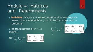
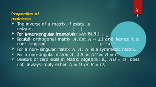
The document outlines a tentative syllabus for a course on matrices and determinants, organized into five modules covering various aspects of calculus and matrix theory. Topics include differentiation and integration techniques, multivariable calculus, properties and operations of matrices, and convergence of sequences and series. Detailed definitions and examples of different types of matrices, properties of determinants, and methods for finding inverses and adjoints are also provided.

![Tentative
syllabus
▶ Module
5:
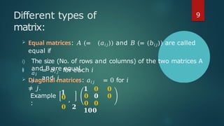
Sequences and Series: Basic ideas on
Sequence; Concept of Monotonic and Bounded
sequence; Convergence and Divergence of Sequence;
Algebra of Sequences (Statement only). Basic idea of an
Infinite Series; Notion of Convergence and Divergence;
Series of Positive T erms - Convergence of infinite G.P.
series and p-series (Statement only); T
ests of
Convergence [Statement only] – Comparison Test,
Integral Test, D’Alembert’s Ratio Test, Raabe’s Test and
Cauchy’s Root test. Alternating Series - Leibnitz’s test
[Statement only], Absolute and Conditional
Convergence.
5](https://image.slidesharecdn.com/mathematicsi-bscm103-module4copy-240803053050-07831f50/85/Mathematics-I-BSCM103-Module-4_copy-pptx-5-320.jpg)
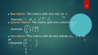
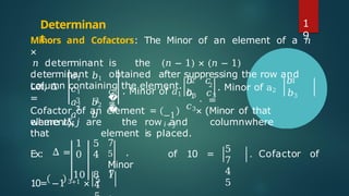
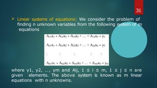

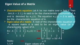
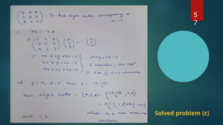
![Let 𝐴 =
(𝑎𝑖𝑗).
Then ᴪ𝐴 𝜆 =
𝑎11 − 𝜆 ⋯
⋮ ⋱
𝑎𝑛1 ⋯
𝑎1𝑛
⋮
𝑎𝑛𝑛
− 𝜆
of the principal
= 𝑐0𝜆𝑛 + 𝑐1𝜆𝑛 −1 + ⋯ + 𝑐𝑛
where 𝑐0 = −1 𝑛 and 𝑐𝑟 = −1 𝑛−𝑟 ×
[sum minors of A order r].
Ex- 𝒄𝟏 = −𝟏 𝒏−𝟏(𝒂𝟏𝟏 + 𝒂𝟐𝟐 + ⋯ + 𝒂𝒏𝒏) = −𝟏
𝒏−𝟏 𝒕𝒓𝒂𝒄𝒆 𝑨 , And
𝒄𝒏 = 𝒅𝒆𝒕𝑨.
The degree of the characteristic equation is same as
4
4](https://image.slidesharecdn.com/mathematicsi-bscm103-module4copy-240803053050-07831f50/85/Mathematics-I-BSCM103-Module-4_copy-pptx-44-320.jpg)
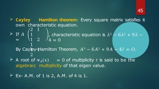
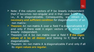
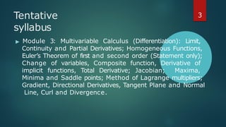
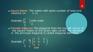
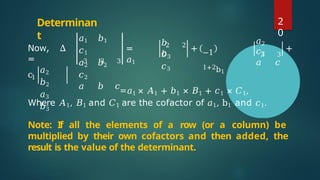
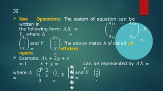
![▶ Since
2 1
1
1 2
1
1 1
2
𝜆1 0
0
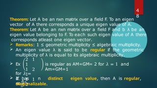
is regular, it is
diagonalizable.
1 0 0
▶ 𝐷 = 0 𝜆2 0 = 0 1 0 .
0 0 𝜆3 0 0 4
▶ 𝑃
=
−1 −1
1
1 0
1
1
1
[1s
t column = eigen vector
corresponding
0
to 𝜆1,
2nd
column = eigen vector corresponding to 𝜆2,
3rd
column = eigen vector corresponding to 𝜆3].
References: B.S. Grewal, STUDY MATERIAL, MATHEMATICS-I (BSCM103), BSH, UEM kolkata
5
2](https://image.slidesharecdn.com/mathematicsi-bscm103-module4copy-240803053050-07831f50/85/Mathematics-I-BSCM103-Module-4_copy-pptx-52-320.jpg)