Downloaded 582 times

![6
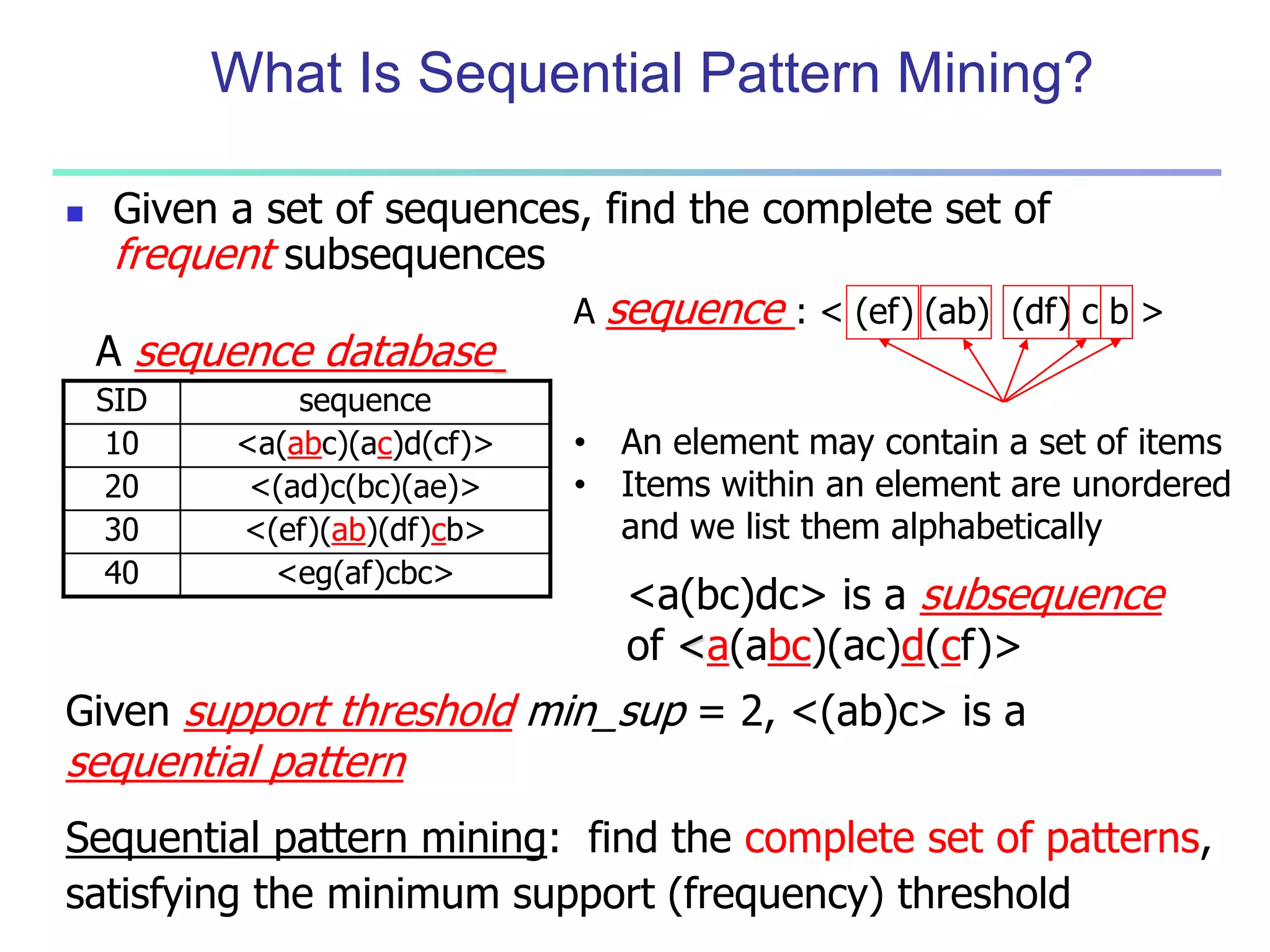
Mining Multiple-Level Association Rules
Items often form hierarchies
Flexible support settings
Items at the lower level are expected to have lower
support
Exploration of shared multi-level mining (Agrawal &
Srikant@VLB’95, Han & Fu@VLDB’95)
uniform support
Milk
[support = 10%]
2% Milk
[support = 6%]
reduced support
Skim Milk
[support = 4%]
Level 1
min_sup = 5%
Level 2
min_sup = 5%
Level 1
min_sup = 5%
Level 2
min_sup = 3%](https://image.slidesharecdn.com/07fpadvanced-140913212112-phpapp02/75/Data-Mining-Concepts-and-Techniques-chapter-07-Advanced-Frequent-Pattern-Mining-6-2048.jpg)
![7
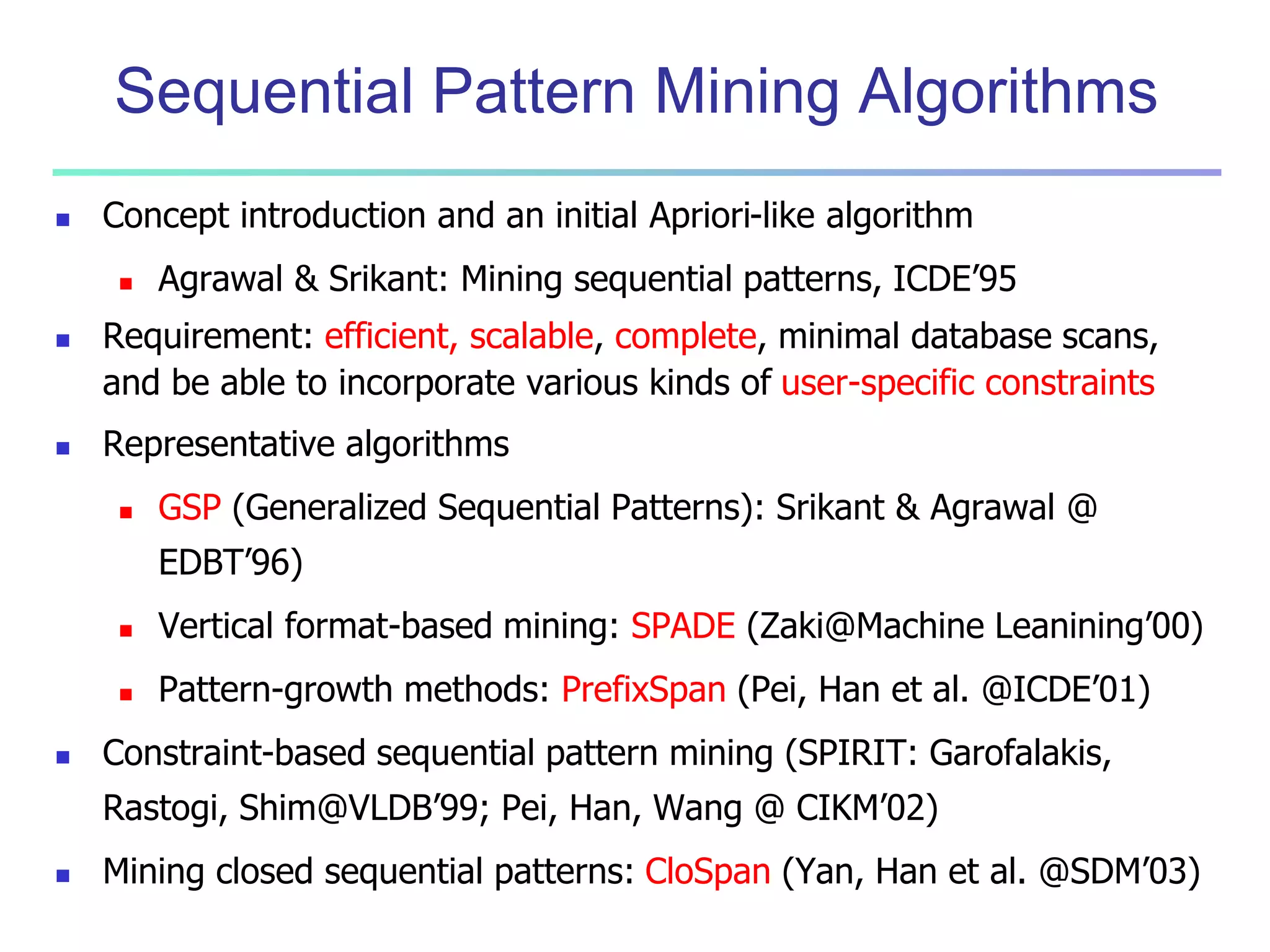
Multi-level Association: Flexible Support and
Redundancy filtering
Flexible min-support thresholds: Some items are more valuable but
less frequent
Use non-uniform, group-based min-support
E.g., {diamond, watch, camera}: 0.05%; {bread, milk}: 5%; …
Redundancy Filtering: Some rules may be redundant due to
“ancestor” relationships between items
milk wheat bread [support = 8%, confidence = 70%]
2% milk wheat bread [support = 2%, confidence = 72%]
The first rule is an ancestor of the second rule
A rule is redundant if its support is close to the “expected” value,
based on the rule’s ancestor](https://image.slidesharecdn.com/07fpadvanced-140913212112-phpapp02/75/Data-Mining-Concepts-and-Techniques-chapter-07-Advanced-Frequent-Pattern-Mining-7-2048.jpg)
![13
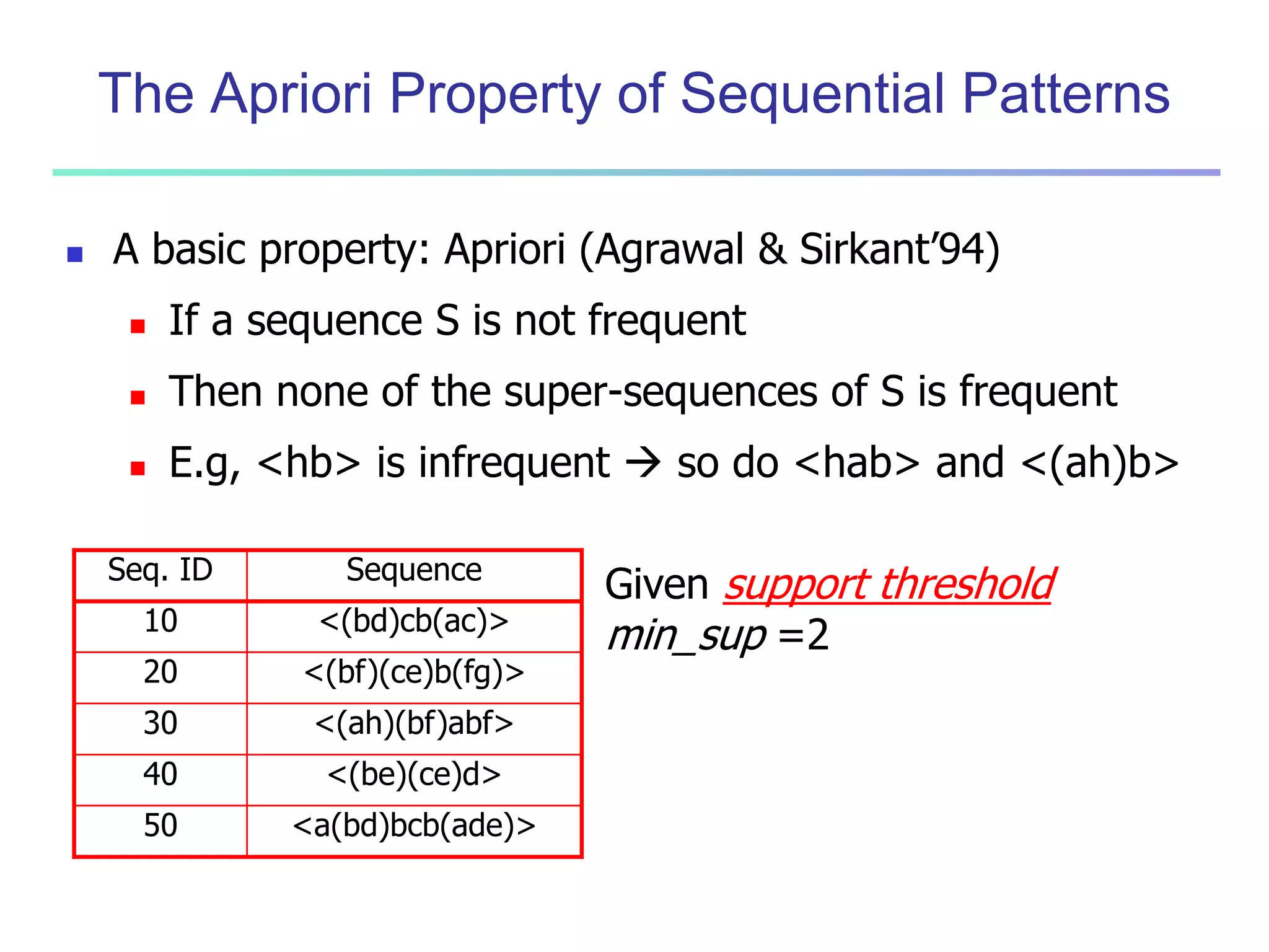
Quantitative Association Rules Based on Statistical
Inference Theory [Aumann and Lindell@DMKD’03]
Finding extraordinary and therefore interesting phenomena, e.g.,
(Sex = female) => Wage: mean=$7/hr (overall mean = $9)
LHS: a subset of the population
RHS: an extraordinary behavior of this subset
The rule is accepted only if a statistical test (e.g., Z-test) confirms the
inference with high confidence
Subrule: highlights the extraordinary behavior of a subset of the pop.
of the super rule
E.g., (Sex = female) ^ (South = yes) => mean wage = $6.3/hr
Two forms of rules
Categorical => quantitative rules, or Quantitative => quantitative rules
E.g., Education in [14-18] (yrs) => mean wage = $11.64/hr
Open problem: Efficient methods for LHS containing two or more
quantitative attributes](https://image.slidesharecdn.com/07fpadvanced-140913212112-phpapp02/75/Data-Mining-Concepts-and-Techniques-chapter-07-Advanced-Frequent-Pattern-Mining-13-2048.jpg)


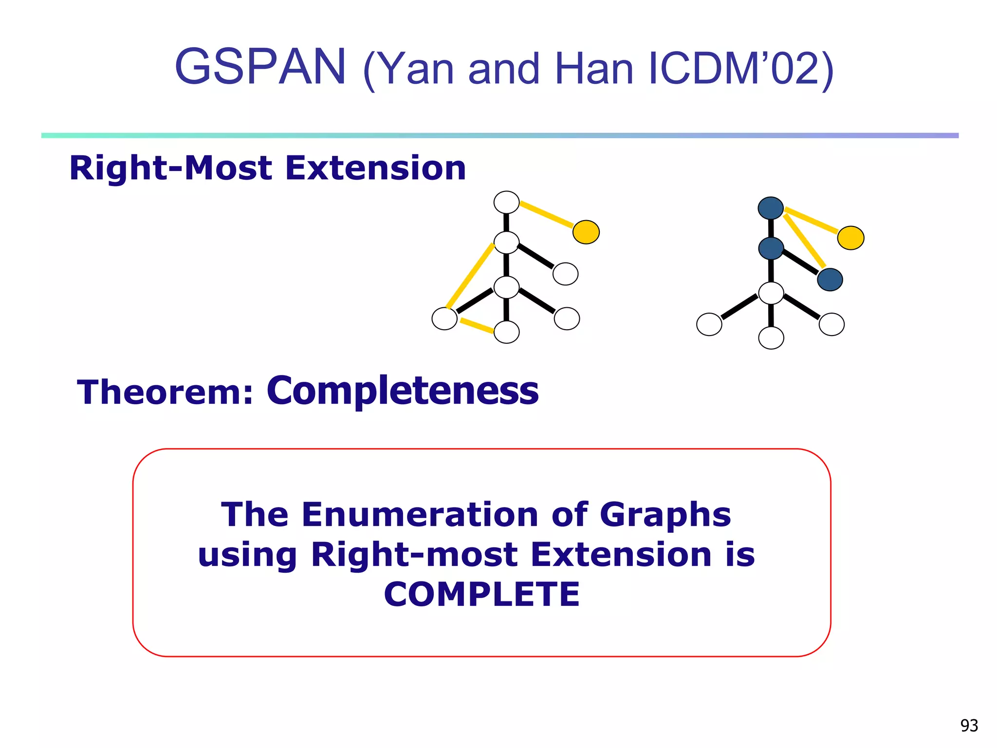
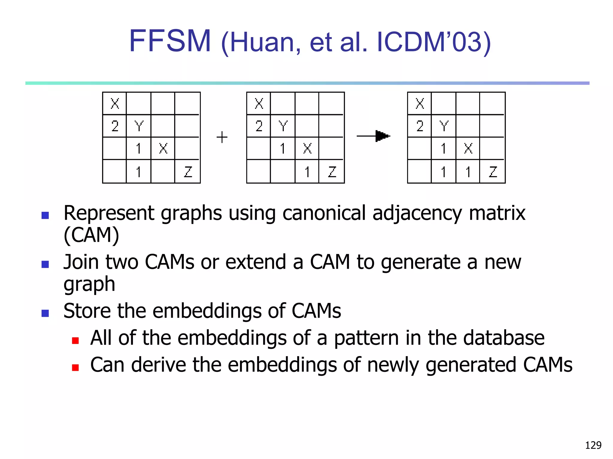
![96
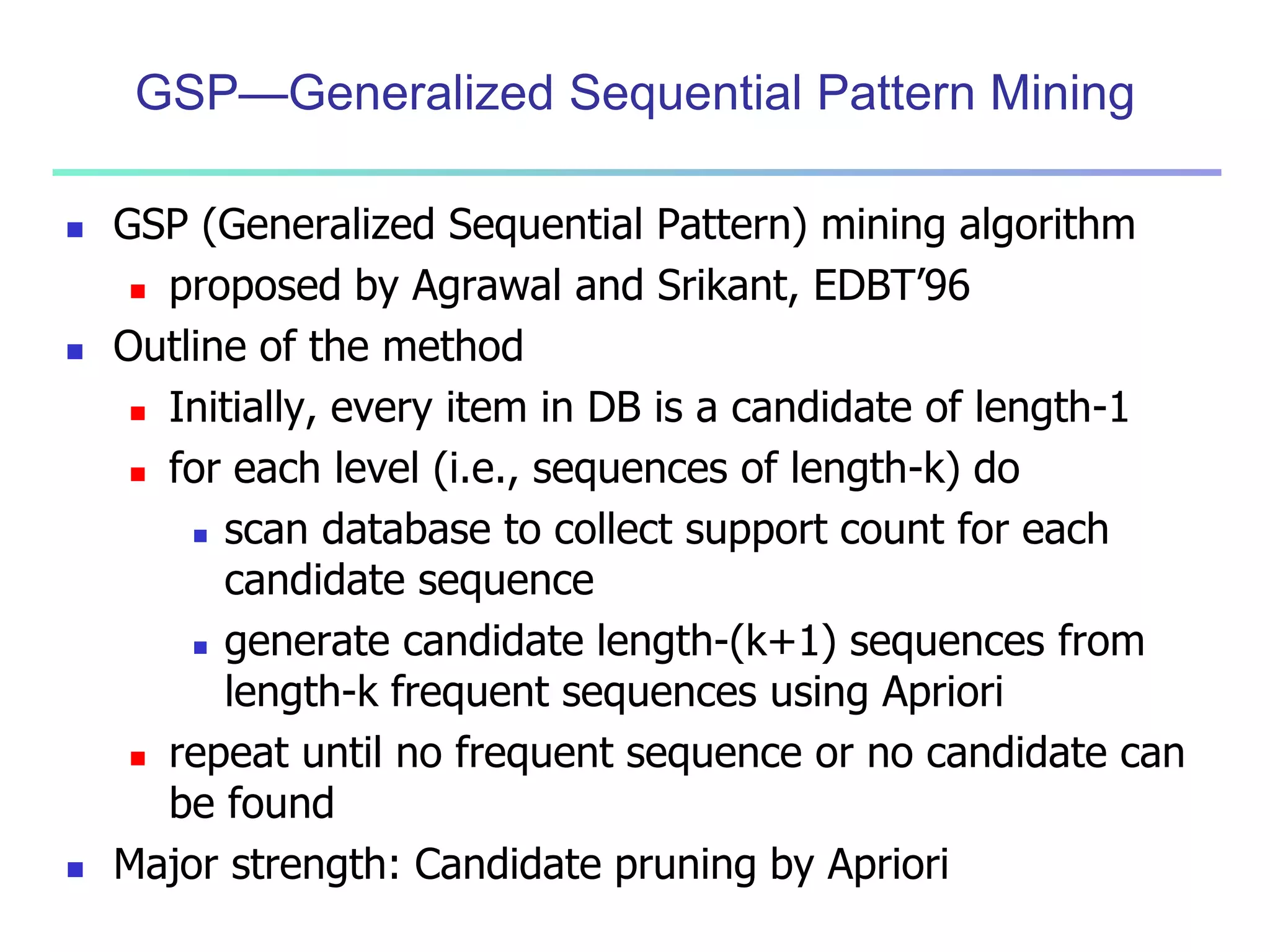
DFS Code Extension
Let a be the minimum DFS code of a graph G and b be
a non-minimum DFS code of G. For any DFS code d
generated from b by one right-most extension,
(i) d is not a minimum DFS code,
(ii) min_dfs(d) cannot be extended from b, and
(iii) min_dfs(d) is either less than a or can be
extended from a.
THEOREM [ RIGHT-EXTENSION ]
The DFS code of a graph extended from a
Non-minimum DFS code is NOT MINIMUM](https://image.slidesharecdn.com/07fpadvanced-140913212112-phpapp02/75/Data-Mining-Concepts-and-Techniques-chapter-07-Advanced-Frequent-Pattern-Mining-95-2048.jpg)

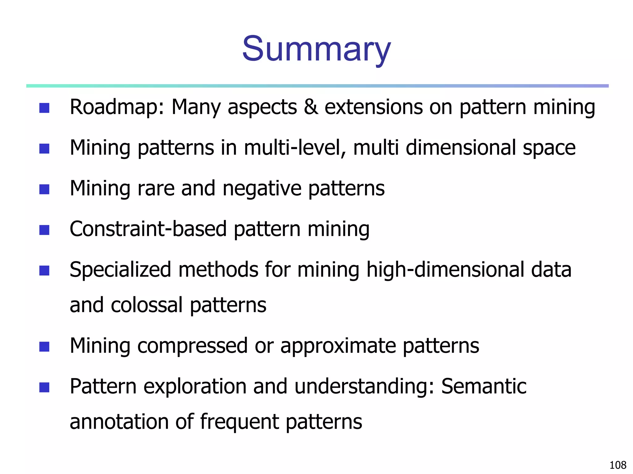


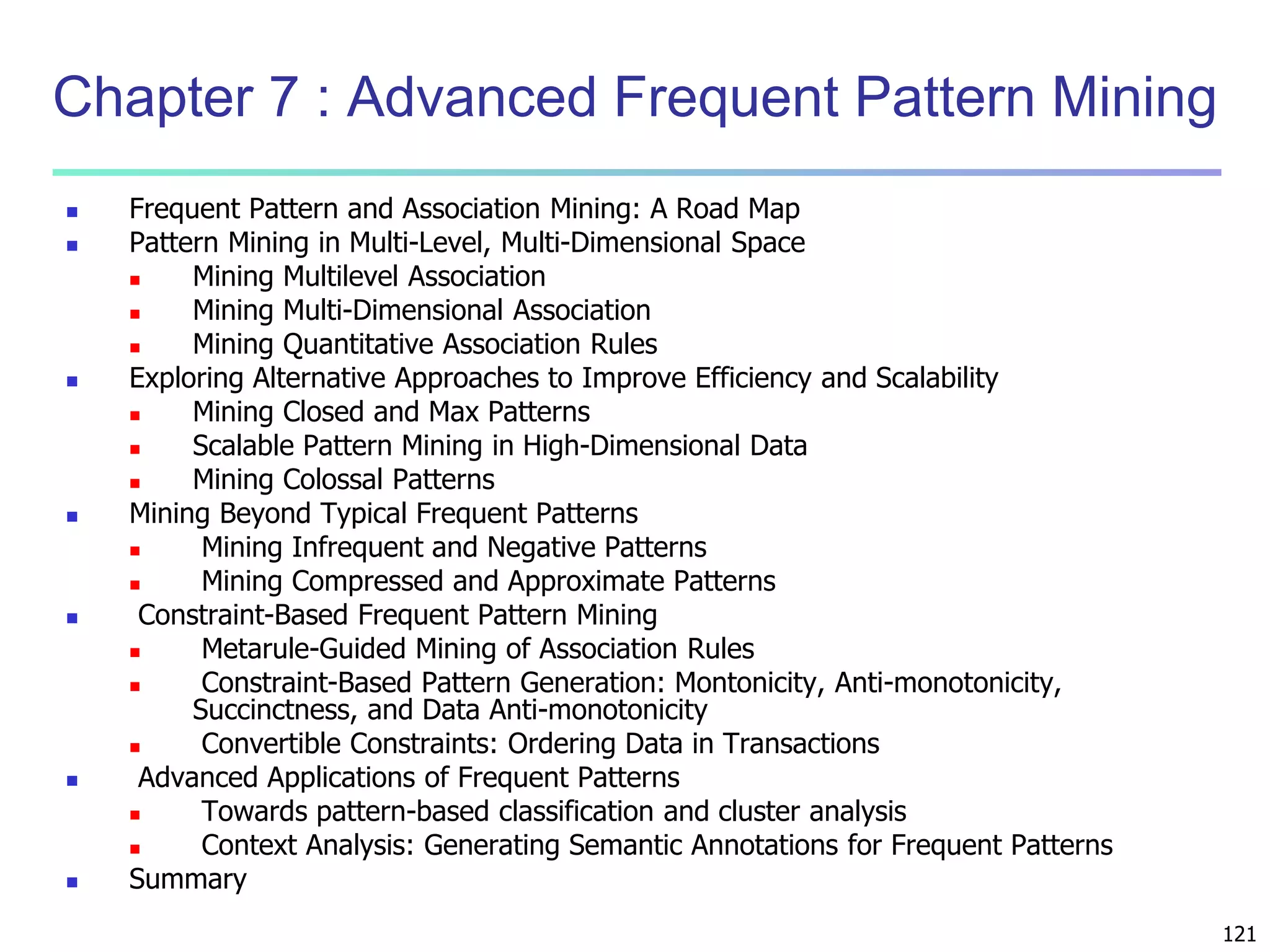

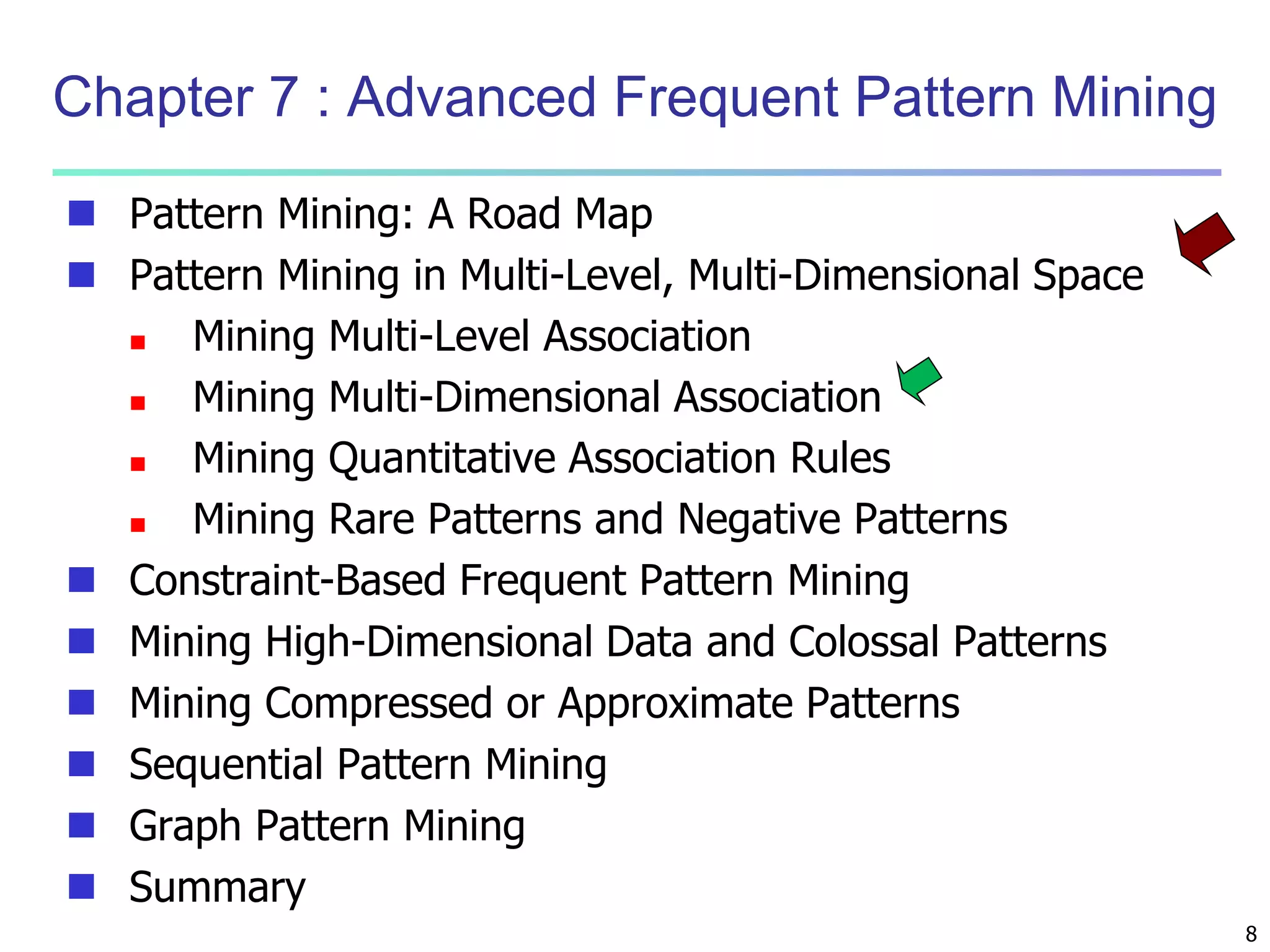
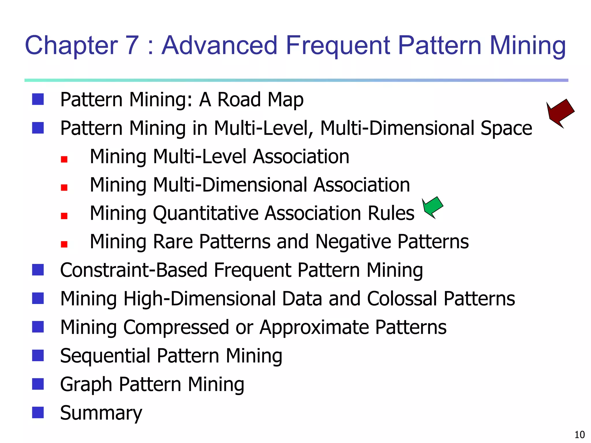
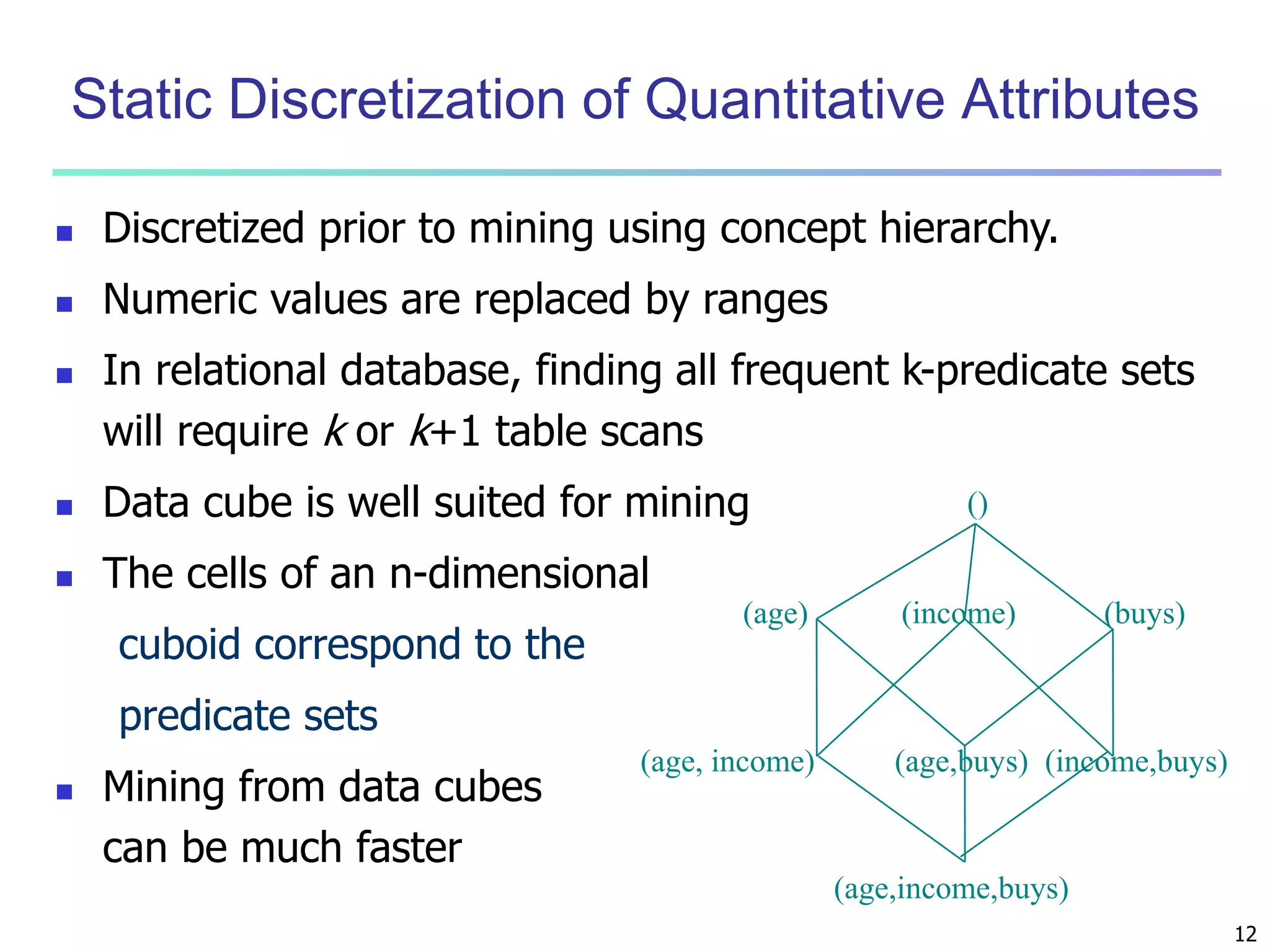
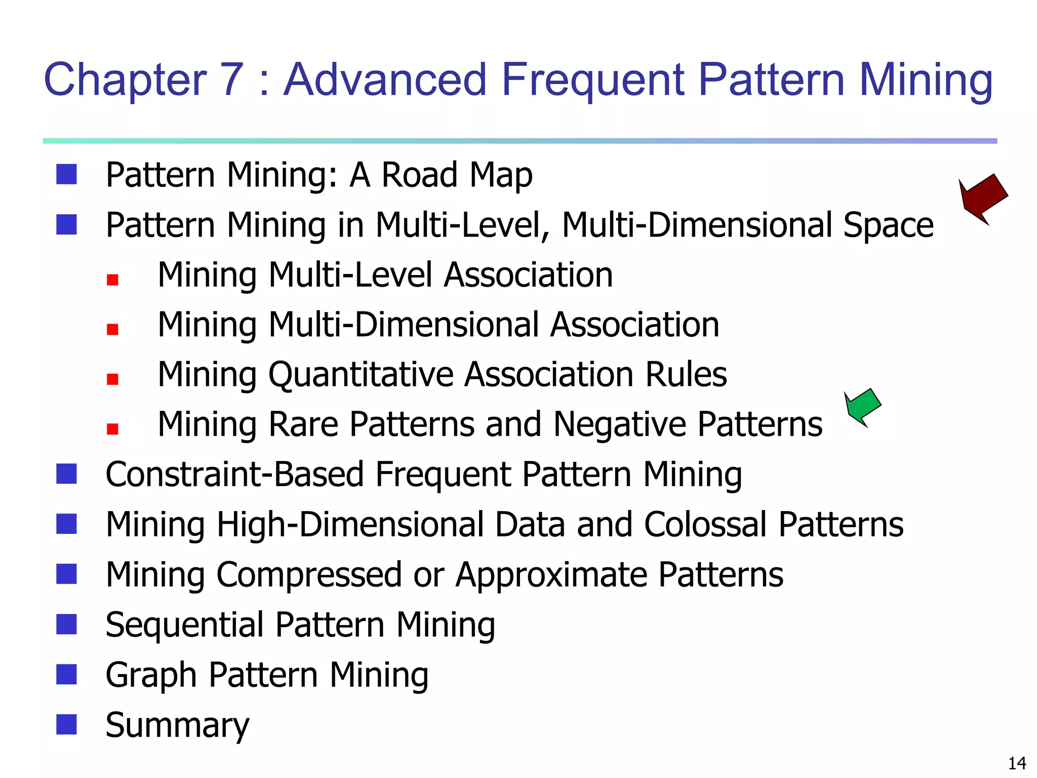
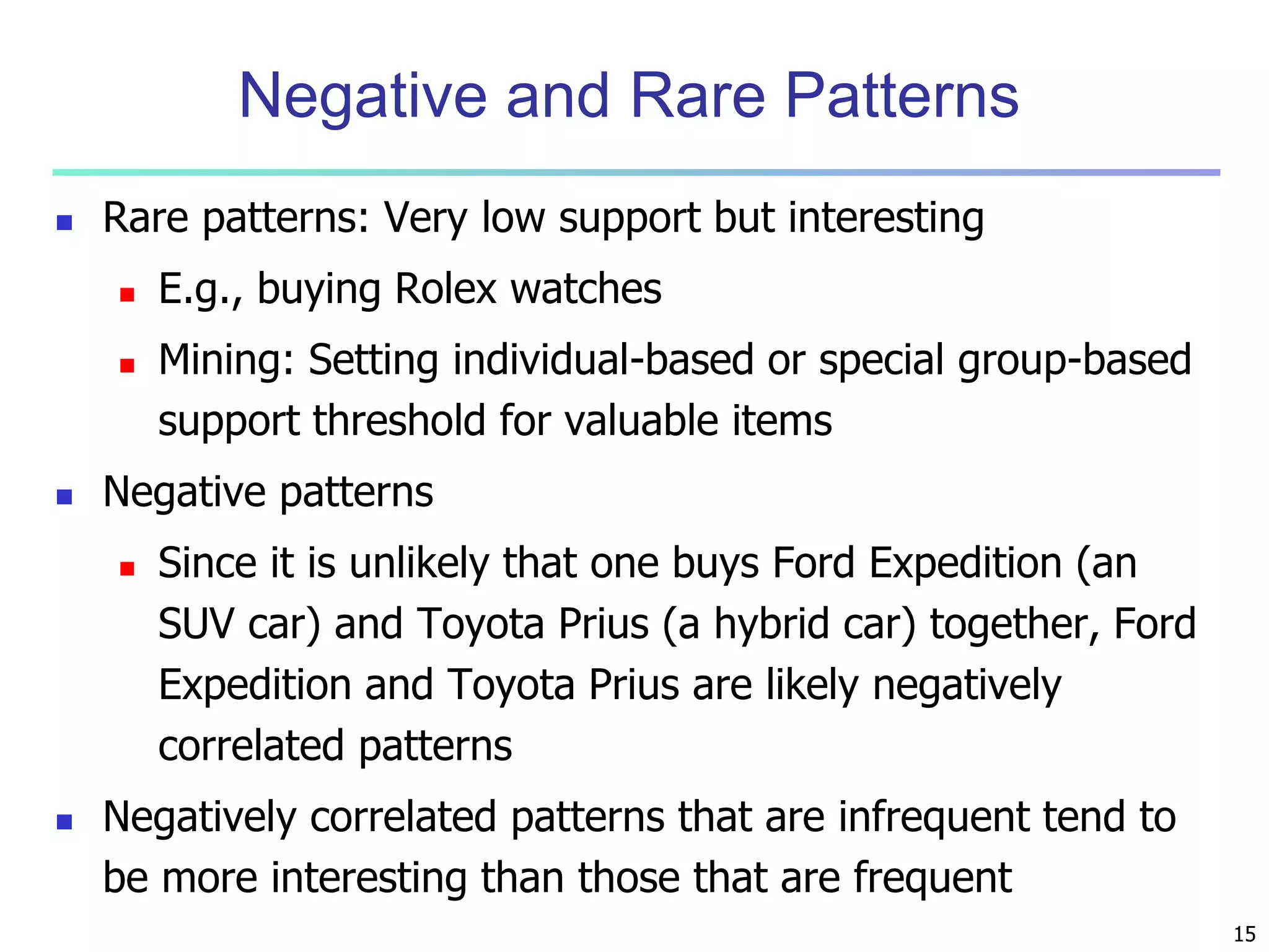
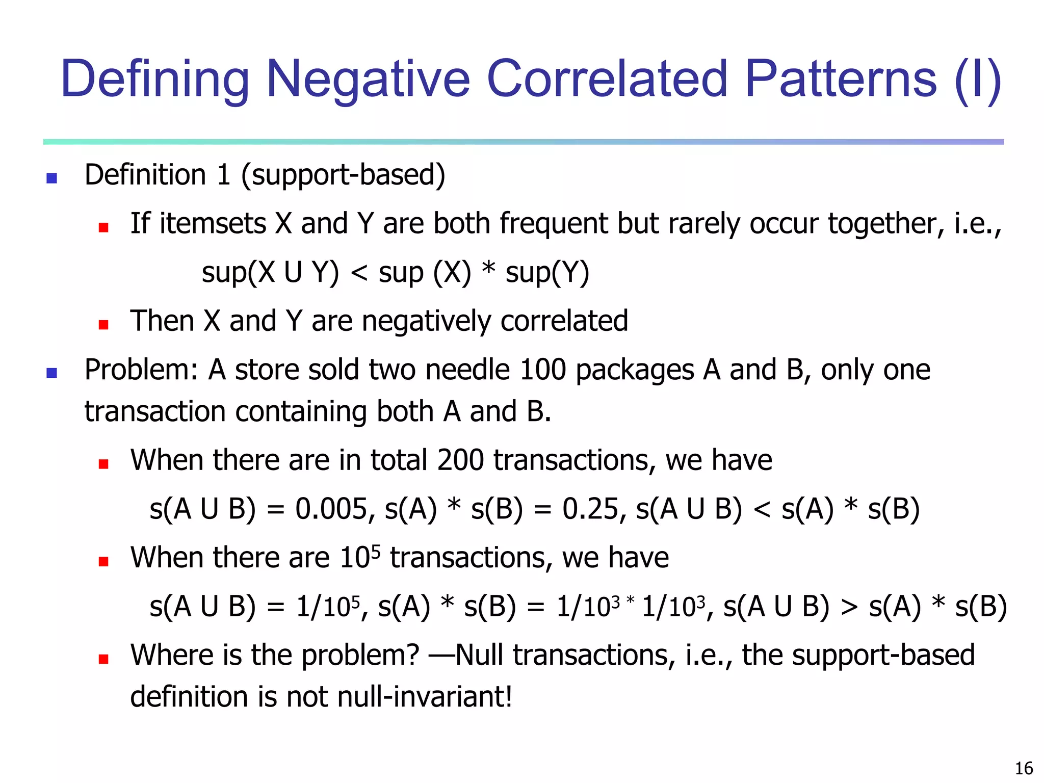
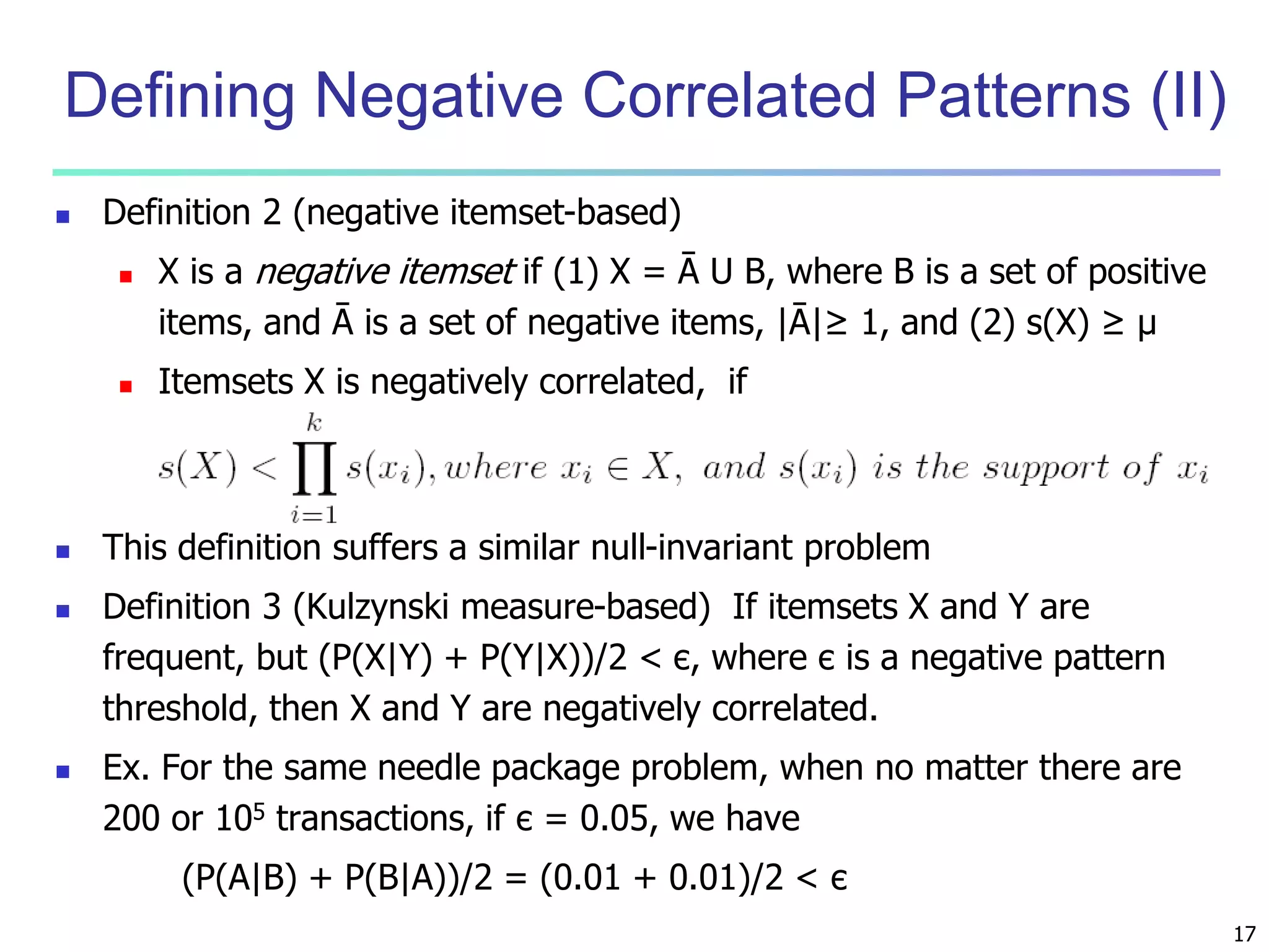
Chapter 7 of 'Data Mining: Concepts and Techniques' discusses advanced frequent pattern mining, covering topics such as multi-level and multi-dimensional pattern mining, mining of quantitative associations, and constraint-based mining. It emphasizes the importance of mining strategies like rare and negative patterns and the necessity of user-directed mining through constraints. Additionally, it addresses efficient data mining techniques and challenges in discovering interesting patterns from vast datasets.


![[BDD 2025 - Artificial Intelligence] Building AI Systems That Users (and Comp...](https://cdn.slidesharecdn.com/ss_thumbnails/ai-buildingaisystemsthatusersandcompanieslove-251124030845-038f7732-thumbnail.jpg?width=640&height=640&fit=bounds)

![[BDD 2025 - Mobile Development] Mobile Engineer and Software Engineer: Are we...](https://cdn.slidesharecdn.com/ss_thumbnails/md-mobileengineerandsoftwareengineerarewestillrelevantsidiqpermana-251127010650-55224ef1-thumbnail.jpg?width=640&height=640&fit=bounds)
![[BDD 2025 - Full-Stack Development] Digital Accessibility: Why Developers nee...](https://cdn.slidesharecdn.com/ss_thumbnails/fs-digitalaccessibilitywhydevelopersneedtoknowandcarein2025-251127011019-0674441d-thumbnail.jpg?width=640&height=640&fit=bounds)


![Support, Monitoring, Continuous Improvement & Scaling Agentic Automation [3/3]](https://cdn.slidesharecdn.com/ss_thumbnails/agenticcommunityseries-day3-cfd-251120170304-ddef8112-thumbnail.jpg?width=640&height=640&fit=bounds)

![[BDD 2025 - Artificial Intelligence] AI for the Underdogs: Innovation for Sma...](https://cdn.slidesharecdn.com/ss_thumbnails/ai-aifortheunderdogsinnovationforsmallbusinesses-251124030839-72a599a4-thumbnail.jpg?width=640&height=640&fit=bounds)

![[BDD 2025 - Full-Stack Development] The Modern Stack: Building Web & AI Appli...](https://cdn.slidesharecdn.com/ss_thumbnails/fs-themodernstackbuildingwebaiapplicationswithserverless-251124030844-388cf04f-thumbnail.jpg?width=640&height=640&fit=bounds)


