Downloaded 283 times


![Better data visualization
5
[resources from en.wikipedia.org]
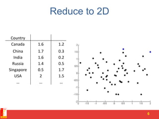
Country
GDP
(trillions of
US$)
Per capita
GDP
(thousands
of intl. $)
Human
Develop-
ment Index
Life
expectancy
Poverty
Index
(Gini as
percentage)
Mean
household
income
(thousands
of US$) …
Canada 1.577 39.17 0.908 80.7 32.6 67.293 …
China 5.878 7.54 0.687 73 46.9 10.22 …
India 1.632 3.41 0.547 64.7 36.8 0.735 …
Russia 1.48 19.84 0.755 65.5 39.9 0.72 …
Singapore 0.223 56.69 0.866 80 42.5 67.1 …
USA 14.527 46.86 0.91 78.3 40.8 84.3 …
… … … … … … …](https://image.slidesharecdn.com/4-pcaandsvr-150730022556-lva1-app6892/85/Dimensionality-reduction-SVD-and-its-applications-5-320.jpg)
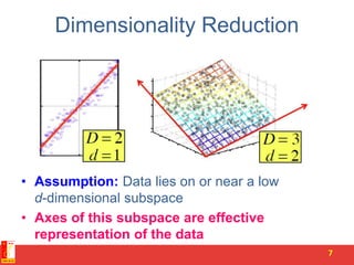
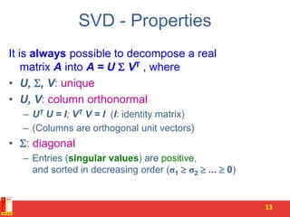
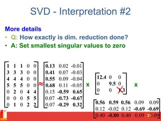
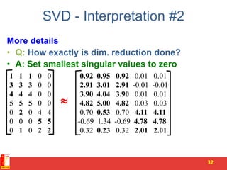
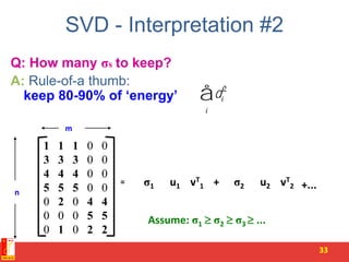
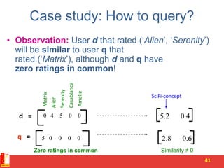
![Rank of a Matrix
• Q: What is rank of a matrix A?
• A: Number of linearly independent columns of A
• For example:
– Matrix A = has rank r=2
• Why? The first two rows are linearly independent, so the rank is at least
2, but all three rows are linearly dependent (the first is equal to the sum of
the second and third) so the rank must be less than 3.
• Why do we care about low rank?
– We can write A as two “basis” vectors: [1 2 1] [-2 -3 1]
– And new coordinates of : [1 0] [0 1] [1 1]
8](https://image.slidesharecdn.com/4-pcaandsvr-150730022556-lva1-app6892/85/Dimensionality-reduction-SVD-and-its-applications-8-320.jpg)
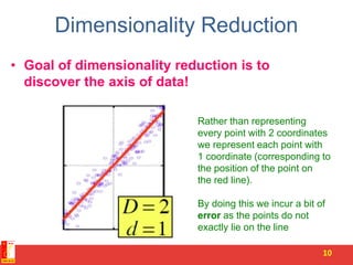
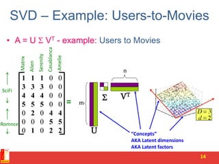
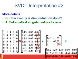
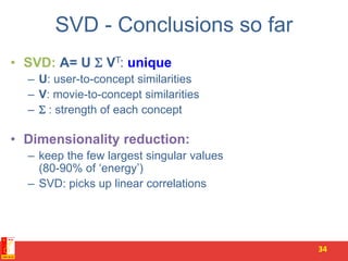
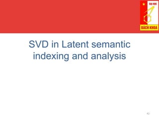
![Rank is “Dimensionality”
• Cloud of points 3D space:
– Think of point positions
as a matrix:
• We can rewrite coordinates more efficiently!
– Old basis vectors: [1 0 0] [0 1 0] [0 0 1]
– New basis vectors: [1 2 1] [-2 -3 1]
– Then A has new coordinates: [1 0]. B: [0 1], C: [1 1]
• Notice: We reduced the number of coordinates!
9
1 row per point:
A
B
C
A](https://image.slidesharecdn.com/4-pcaandsvr-150730022556-lva1-app6892/85/Dimensionality-reduction-SVD-and-its-applications-9-320.jpg)
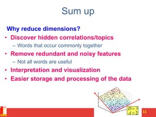
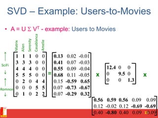
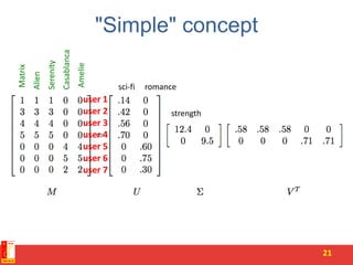
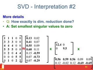
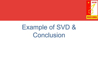
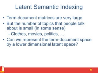
![SVD - Definition
A[m x n] = U[m x r] [ r x r] (V[n x r])T
• A: Input data matrix
– m x n matrix (e.g., m documents, n terms)
• U: Left singular vectors
– m x r matrix (m documents, r concepts)
• : Singular values
– r x r diagonal matrix (strength of each ‘concept’)
(r : rank of the matrix A)
• V: Right singular vectors
– n x r matrix (n terms, r concepts)
12](https://image.slidesharecdn.com/4-pcaandsvr-150730022556-lva1-app6892/85/Dimensionality-reduction-SVD-and-its-applications-12-320.jpg)


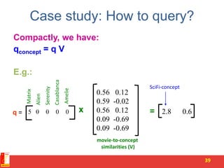


![PCA algorithm
50
Reduce data from -dimensions to -dimensions
Compute “covariance matrix”:
Compute “eigenvectors” of matrix :
[U,S,V] = svd(Sigma);](https://image.slidesharecdn.com/4-pcaandsvr-150730022556-lva1-app6892/85/Dimensionality-reduction-SVD-and-its-applications-50-320.jpg)
![51
From , we get:[U,S,V] = svd(Sigma)](https://image.slidesharecdn.com/4-pcaandsvr-150730022556-lva1-app6892/85/Dimensionality-reduction-SVD-and-its-applications-51-320.jpg)

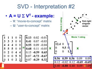
SVD (singular value decomposition) is a technique for dimensionality reduction that decomposes a matrix A into three matrices: U, Σ, and V. U and V are orthogonal matrices that represent the left and right singular vectors of A. Σ is a diagonal matrix containing the singular values of A in descending order. SVD can be used to reduce the dimensionality of data by projecting it onto only the first few principal components represented by the top singular vectors in U and V. This provides an interpretation of the data in a lower dimensional space while minimizing reconstruction error.