The document discusses different methods for fitting equations to data, including interpolating polynomials, least squares fitting, and examples of non-polynomial forms. It provides sample MATLAB code for finding an interpolating polynomial that passes through every data point in a sample data set, as well as code for performing a cubic least squares fit. The document concludes by giving practice problems involving fitting equations to saturation property data for water.

1. Last modified:January 1, 1970 GMT
An Introduction to Matlab(tm): Lesson 8
EQUATION FITTING
Many occasions arise when we have a set of (x,y) pairs and we
desire to find an equation or function that "fits" these data. The
procedure we follow can be generally classified in one of two
categories, interpolating functions or least squares functions.
The least-squares function is one that obtains the best fit,
where the meaning here of "best" is based on minimizing the sum of
the squares of the differences between the function and the data
pairs. Clearly the idea of "least squares" is to achieve some sort
of average or mean value function whose graphical curve does not
typically pass through any of the (x,y) data pairs. It is
appropriate for experimental data in which every data pair is
obtained under conditions of uncertainty and for which any
collected data, as a consequence of experimental error, may be
greater or less than the true value.
INTERPOLATING POLYNOMIAL
The interpolating function is one that satisfies every data
point exactly. When viewed in a graphical plot, the interpolating
function passes through each data point. If for convenience we
select the polynomial form as the function, a polynomial of degree
'n' can be found for a set of 'n+1' (x,y) data pairs. The general
form of the polynomial can be written
y = a0 + a1x + a2x2 + a3x3 + ....... + anxn
To evaluate the interpolating polynomial of degree 'n' for any data
set, we must evaluate 'n+1' coefficients, a0, a1, a2, a3, .....an.
Given the 'n+1' (x,y) data pairs, we can form 'n+1' equations
y1
y2
y3
.
.
.
= a0 + a1x1 + a2x12 + a3x13 + ...... + anx1n
= a0 + a1x2 + a2x22 + a3x23 + ...... + anx2n
= a0 + a1x3 + a2x32 + a3x33 + ...... + anx3n
. .
.
.
.
. .
.
.
.
. .
.
.
.
yn+1 = a0 + a1xn+1 + a2xn+12 + a3xn+13 + ... + anxn+1n

2. This is a solvable set of 'n+1' equations with 'n+1' unknowns. The
unknowns are the coefficients a0, a1,......an. If there exists only
two or three equations, the solution procedure for the unknown
coefficients can conveniently follow Cramer's Rule. In general,
however, it is common to rely on matrix algebra to manipulate these
equations into a format for which n operations of back substitution
will obtain the unknown coefficients. Here we will simply rely on
the methods of right (or left) division in 'matlab' to obtain the
unknown coefficients, leaving the details of the numerical method
for back substitution for later discussion.
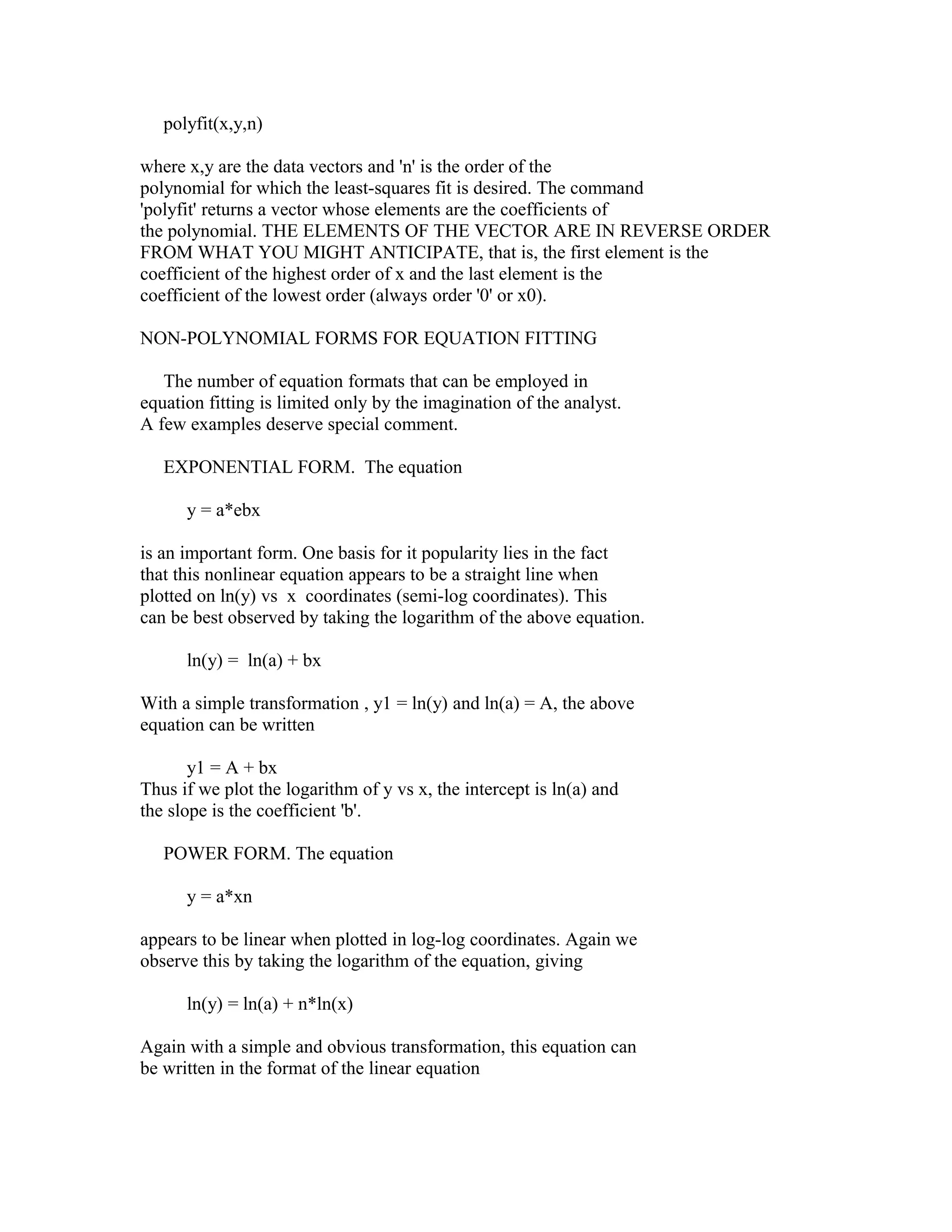
Note that the set of equations can be conveniently expressed
by the matrix equation
[y] = [X][a]
where
y1
1
x1 x12.....x1n+1
y2
1
[y] =
[X] =
y3
1
.
. .
.
. .
.
. .
yn+1
1
a1
x2 x22.....x2n+1
a2
[a] =
x3 x32.....x3n+1
a3
.
.
.
.
.
.
.
.
.
xn+1 xn+12... xn+1n+1
an+1
Note that the right side of the matrix equation must be the product
of a 'n+1' x 'n+1' square matrix times a 'n+1' x 1 column matrix!
The solution using Gauss elimination calls for left division in
'matlab' or
[a] = [X][y]
Using this method, we can find the coefficients for a n-degree
polynomial that passes exactly through 'n+1' data points.
If we have a large data set, each data pair including some
experimental error, the n-degree polynomial is NOT A GOOD CHOICE.
Polynomials of degree larger than five or six often have terribly
unrealistic behavior BETWEEN the data points even though the
polynomial curve passes through every data point ! As an example,
consider these data.
x
y

3. 2
3
4
5
6
7
8
9
10
4
3
5
4
7
5
7
10
9
There are 9 data points in this set. It is clear that as x
increases, so also does y increase; however, it appears to be doing
so in a nonlinear way. Let's see what the data looks like. In
'matlab', create two vectors for these data.
x9 = [2:1:10];
y9 = [ 4 3 5 4 7 5 7 10 9 ];
To observe these data plotted as points, execute
plot(x9,y9,'o')
Because we have nine data pairs, it is possible to construct an
eighth-degree interpolating polynomial.
y = a0 + a1x + a2x2 + a3x3 + ....... + a8x8
To find the unknown coefficients, define the column vector y
y = y9'
and the matrix X
X = [ones(1,9);x9;x9.^2;x9.^3;x9.^4;x9.^5;x9.^6;x9.^7;x9.^8]'
Note that X is defined using the transpose, the ones() function and
the array operator ' .^ '. With X and y so defined, they satisfy
the equation
[X][a] = [y]
Solve for the coefficients, matrix a in the above equation, by
entering the command

4. a = Xy
which results in
a = [ 1.0e+003*
3.8140
-6.6204
4.7831
-1.8859
.4457
- .0649
.0057
- .0003
.0000 ]
Note that the ninth coefficient a(8) appears to be zero. Actually,
it is finite, it only appears to be zero because 'matlab' is
printing only 4 significant figures to the left of the decimal
point. To observe the coefficients with more significant figures,
enter the commands
format long
a
and the format is changed to one with 15 significant digits.
Clearly a(8) is not zero, it is a small number because it is
multiplying a number, x, raised to the eight power.
Now that we have the coefficients, let's generate a
sufficient number of points to create a smooth curve. For x, form
a vector over the range 2 <= x <= 10 in increments of 0.1.
x = [ 2:.1:10 ];
For y, calculate the value of the eighth degree polynomial for each
x.
y =a(1)+ a(2).*x + a(3).*x.^2 + a(4).*x.^3 + a(5).*x.^4...
+ a(6).*x.^5 + a(7).*x.^6 + a(8).*x.^7 + a(9).*x.^8;
Now plot (x,y) and the data points (x9,y9).
plot(x,y,x9,y9,'o')
The polynomial results appear to pass exactly through every data
point, but clearly the polynomial is useless for representing our

5. impression of the data at any other point within the range of x!
This is a common behavior for high-order interpolating polynomials.
For this reason, one should never attempt to use high order
interpolating polynomials to represent experimental data.
LEAST SQUARES
A lower order polynomial, possibly a cubic polynomial might be
a sufficient choice; however, a cubic polynomial would have 4
unknown coefficients and we have 9 data points. Which four of the
nine do we select? The method of least squares responds to this
problem by taking an "average" or best curve that includes
information from every one of the data points. The method is well
explained in Chapter 3 of the text, EXPERIMENTAL METHODS FOR
ENGINEERS by J. P. Holman. The details will not be repeated here;
however, the text specializes the result to a first and second
order polynomials. Here we would like to retain the polynomial
format and express the result for the third degree polynomial. If
we desire a quadratic or linear equation, it is easy to select the
reduced matrices that create the desired coefficients. Thus we
find that for the equation
y = a0 + a1x + a2x2 + a3x3
the four unknown coefficients are evaluated from
a=XB
where
a0
m ‘xi ‘xi2 ‘xi3
‘yi
a1
‘xi ‘xi2 ‘xi3 ‘xi4
‘xiyi
[a] =
[X] =
[B] =
a2
‘xi2 ‘xi3 ‘xi4 ‘xi5
‘xi2yi
a3
‘xi3 ‘xi4 ‘xi5 ‘xi6
‘xi3yi
The summation is over the range 1 to m, where m is the number of
(x,y) data pairs. Note that for any least-squares equation fit,
you must have at least one more data point than unknown
coefficients, or m > n+1.
MATLAB FUNCTION FOR LEAST SQUARES
There is a convenient function in 'matlab' for polynomial
equation fitting with the method of least squares. The command is

6. polyfit(x,y,n)
where x,y are the data vectors and 'n' is the order of the
polynomial for which the least-squares fit is desired. The command
'polyfit' returns a vector whose elements are the coefficients of
the polynomial. THE ELEMENTS OF THE VECTOR ARE IN REVERSE ORDER
FROM WHAT YOU MIGHT ANTICIPATE, that is, the first element is the
coefficient of the highest order of x and the last element is the
coefficient of the lowest order (always order '0' or x0).
NON-POLYNOMIAL FORMS FOR EQUATION FITTING
The number of equation formats that can be employed in
equation fitting is limited only by the imagination of the analyst.
A few examples deserve special comment.
EXPONENTIAL FORM. The equation
y = a*ebx
is an important form. One basis for it popularity lies in the fact
that this nonlinear equation appears to be a straight line when
plotted on ln(y) vs x coordinates (semi-log coordinates). This
can be best observed by taking the logarithm of the above equation.
ln(y) = ln(a) + bx
With a simple transformation , y1 = ln(y) and ln(a) = A, the above
equation can be written
y1 = A + bx
Thus if we plot the logarithm of y vs x, the intercept is ln(a) and
the slope is the coefficient 'b'.
POWER FORM. The equation
y = a*xn
appears to be linear when plotted in log-log coordinates. Again we
observe this by taking the logarithm of the equation, giving
ln(y) = ln(a) + n*ln(x)
Again with a simple and obvious transformation, this equation can
be written in the format of the linear equation

7. y1 = A + n*x1
Of course it is convenient to obtain least squares curves of these
forms by first applying the transformation to the data, and then
fitting the linear equation to the transformed data.
HYPERBOLIC FORM. The hyperbolic equation
y = a + b/x
appears to be linear when y is plotted versus 1/x rather than x.
This equation is sometimes useful when data exhibits a decreasing
value of y as x increases.
ASYMPTOTES. The hyperbolic form above exhibits an asymptote.
As x Π, y a . Asymptotes may exist for either variable, x or
y. If an asymptote can be recognized from knowledge of the physics
in the problem, it will facilitate the equation fitting process if
a transformation is introduced. For example, in the hyperbolic
equation
y = a + b/x
the transformation z = y - a results in
z = b/x
which eliminates one of the unknown parameters in the equation
fitting problem.
PRACTICE PROBLEMS
SATURATION PROPERTIES OF WATER
TEMP(C) PRESSURE(kPa) SPEC.VOL(m3/kg) ENTHALPY-hg(kJ/kg)
0 .6108
206.3
2501.6
10 1.227
106.4
2519.9
20 2.337
57.84
2538.2
30 4.241
32.93
2556.4
40 7.375
19.55
2574.4
50 12.335
12.05
2592.2

8. 60
70
80
90
100
19.92
31.16
47.36
70.11
101.33
7.679
5.046
3.409
2.361
1.673
2609.7
2626.9
2643.8
2660.1
2676.0
1. Using the above data and linear interpolation, calculate the
saturation pressure at 65 C. Next, find the interpolating
polynomial that satisfies the above data for saturation temperature
and pressure for 50, 60 and 70 C. Using this polynomial, compute
the saturation pressure at 65 C and compare the result with your
linear interpolation.
2. Find the interpolating polynomial that satisfies exactly the
above data for saturation temperature and specific volume for the
temperatures 10, 20 and 30 C. Using this polynomial, compute the
specific volume at a temperature of 15 C and compare the result
with linear interpolation from the table.
3. A function is expected to be of the form y = axn. Two data
points are available to evaluate the unknown coefficient a, and
exponent n. The data are (100,50) and (1000,10). Find the
parameters a and n.
4. (a) Find the linear equation using least-squares that represents
the temperature-enthalpy data in the above table. ( h = h(T) )
(b) Find a second-degree polynomial that represents the Tenthalpy data in the above table using the method of least squares.
(c) Plot the (h,T) data and the above two equations.
5. Find the unknown coefficients in the below equation that
represents the T-p data in the above table.
ln(p) = A + B/T
Plot the data and the equation.
6. (a) Find the 1st, 2nd and 3rd order polynomials that satisfy the
p vs. T data above, and plot them on a single graphics for
comparison.
(b) Prepare a graphic plot that compares the result of (5.) above
with the 3rd order equation found in 6(a.).
Back to Matlab In-House Tutorials