MIT OpenCourseWare provides course materials for the free online course 6.094 Introduction to MATLAB taught in January 2009. The course covers topics like linear algebra, polynomials, optimization, differentiation and integration, and solving differential equations using MATLAB. Lecture 3 focuses on solving systems of linear equations, matrix operations, polynomial fitting to data, nonlinear root finding, function minimization, and numerical methods for differentiation, integration, and solving ordinary differential equations.

1. MIT OpenCourseWare
http://ocw.mit.edu
6.094 Introduction to MATLAB®
January (IAP) 2009
For information about citing these materials or our Terms of Use, visit: http://ocw.mit.edu/terms.

2. 6.094
Introduction to Programming in MATLAB®
Lecture 3 : Solving Equations and Curve Fitting
Sourav Dey
Danilo Šćepanović
Ankit Patel
Patrick Ho
IAP 2009

3. Outline
(1) Linear Algebra
(2) Polynomials
(3) Optimization
(4) Differentiation/Integration
(5) Differential Equations

4. Systems of Linear Equations
• Given a system of linear equations MATLAB makes linear
x+2y-3z=5
algebra fun!
-3x-y+z=-8
x-y+z=0
• Construct matrices so the system is described by Ax=b
» A=[1 2 -3;-3 -1 1;1 -1 1];
» b=[5;-8;0];
• And solve with a single line of code!
» x=Ab;
x is a 3x1 vector containing the values of x, y, and z
• The will work with square or rectangular systems.
• Gives least squares solution for rectangular systems. Solution
depends on whether the system is over or underdetermined.

5. More Linear Algebra
• Given a matrix
» mat=[1 2 -3;-3 -1 1;1 -1 1];
• Calculate the rank of a matrix
» r=rank(mat);
the number of linearly independent rows or columns
• Calculate the determinant
» d=det(mat);
mat must be square
if determinant is nonzero, matrix is invertible
• Get the matrix inverse
» E=inv(mat);
if an equation is of the form A*x=b with A a square matrix,
x=Ab is the same as x=inv(A)*b

6. Matrix Decompositions
• MATLAB has built-in matrix decomposition methods
• The most common ones are
» [V,D]=eig(X)
Eigenvalue decomposition
» [U,S,V]=svd(X)
Singular value decomposition
» [Q,R]=qr(X)
QR decomposition

7. Exercise: Linear Algebra
• Solve the following systems of equations:
System 1:
x+4y=34
-3x+y=2
System 2:
2x-2y=4
-x+y=3
3x+4y = 2

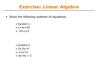
8. Exercise: Linear Algebra
• Solve the following systems of equations:
System 1: » A=[1 4;-3 1];
x+4y=34 » b=[34;2];
-3x+y=2 » rank(A)
» x=inv(A)*b;
System 2: » A=[2 -2;-1 1;3 4];
2x-2y=4 » b=[4;3;2];
-x+y=3 » rank(A)
3x+4y = 2 rectangular matrix
» x1=Ab;
gives least squares solution
» A*x1

9. Outline
(1) Linear Algebra
(2) Polynomials
(3) Optimization
(4) Differentiation/Integration
(5) Differential Equations

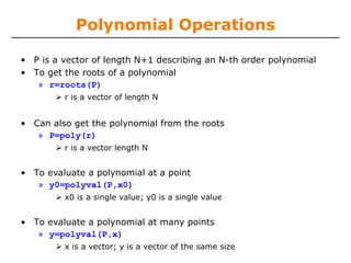
10. Polynomials
• Many functions can be well described by a high-order
polynomial
• MATLAB represents a polynomials by a vector of coefficients
if vector P describes a polynomial
– ax3+bx2+cx+d
P(1) P(2) P(3) P(4)
• P=[1 0 -2] represents the polynomial x2-2
• P=[2 0 0 0] represents the polynomial 2x3

11. Polynomial Operations
• P is a vector of length N+1 describing an N-th order polynomial
• To get the roots of a polynomial
» r=roots(P)
r is a vector of length N
• Can also get the polynomial from the roots
» P=poly(r)
r is a vector length N
• To evaluate a polynomial at a point
» y0=polyval(P,x0)
x0 is a single value; y0 is a single value
• To evaluate a polynomial at many points
» y=polyval(P,x)
x is a vector; y is a vector of the same size

12. Polynomial Fitting
• MATLAB makes it very easy to fit polynomials to data
• Given data vectors X=[-1 0 2] and Y=[0 -1 3]
» p2=polyfit(X,Y,2);
finds the best second order polynomial that fits the points
(-1,0),(0,-1), and (2,3)
see help polyfit for more information
» plot(X,Y,’o’, ‘MarkerSize’, 10);
» hold on;
» x = linspace(-2,2,1000);
» plot(x,polyval(p2,x), ‘r--’);

13. Exercise: Polynomial Fitting
• Evaluate x^2 over x=-4:0.1:4 and save it as y.
• Add random noise to these samples. Use randn. Plot the
noisy signal with . markers
• fit a 2nd degree polynomial to the noisy data
• plot the fitted polynomial on the same plot, using the same
x values and a red line

14. Exercise: Polynomial Fitting
• Evaluate x^2 over x=-4:0.1:4 and save it as y.
» x=-4:0.1:4;
» y=x.^2;
• Add random noise to these samples. Use randn. Plot the
noisy signal with . markers
» y=y+randn(size(y));
» plot(x,y,’.’);
• fit a 2nd degree polynomial to the noisy data
» [p]=polyfit(x,y,2);
• plot the fitted polynomial on the same plot, using the same
x values and a red line
» hold on;
» plot(x,polyval(p,x),’r’)

15. Outline
(1) Linear Algebra
(2) Polynomials
(3) Optimization
(4) Differentiation/Integration
(5) Differential Equations

16. Nonlinear Root Finding
• Many real-world problems require us to solve f(x)=0
• Can use fzero to calculate roots for any arbitrary function
• fzero needs a function passed to it.
• We will see this more and more as we delve into solving
equations.
• Make a separate function file
» x=fzero('myfun',1)
» x=fzero(@myfun,1)
1 specifies a
point close to
the root
Courtesy of The MathWorks, Inc. Used with permission.

17. Minimizing a Function
• fminbnd: minimizing a function over a bounded interval
» x=fminbnd('myfun',-1,2);
myfun takes a scalar input and returns a scalar output
myfun(x) will be the minimum of myfun for -1≤x ≤ 2
• fminsearch: unconstrained interval
» x=fminsearch('myfun',.5)
finds the local minimum of myfun starting at x=0.5

18. Anonymous Functions
• You do not have to make a separate function file
• Instead, you can make an anonymous function
» x=fzero(@(x)(cos(exp(x))+x^2-1), 1 );
input function to evaluate
» x=fminbnd(@(x) (cos(exp(x))+x^2-1),-1,2);

19. Optimization Toolbox
• If you are familiar with optimization methods, use the
optimization toolbox
• Useful for larger, more structured optimization problems
• Sample functions (see help for more info)
» linprog
linear programming using interior point methods
» quadprog
quadratic programming solver
» fmincon
constrained nonlinear optimization

20. Exercise: Min-Finding
Find the minimum of the function f(x) =
cos(4*x).*sin(10*x).*exp(-abs(x)) over the range –pi to
pi. Use fminbnd. Is your answer really the minimum
over this range?

21. Exercise: Min-Finding
Find the minimum of the function f(x) =
cos(4*x).*sin(10*x).*exp(-abs(x)) over the range –pi to
pi. Use fminbnd. Is your answer really the minimum
over this range?
function y = myFun(x)
y=cos(4*x).*sin(10*x).*exp(-abs(x));
fminbnd(‘myFun’, -pi, pi);

22. Outline
(1) Linear Algebra
(2) Polynomials
(3) Optimization
(4) Differentiation/Integration
(5) Differential Equations

23. Numerical Differentiation
1
• MATLAB can 'differentiate' numerically
0.8
» x=0:0.01:2*pi; 0.6
0.4
» y=sin(x); 0.2
» dydx=diff(y)./diff(x); 0
diff computes the first difference -0.2
-0.4
-0.6
• Can also operate on matrices -0.8
» mat=[1 3 5;4 8 6]; -1
0 100 200 300 400 500 600 700
» dm=diff(mat,1,2)
first difference of mat along the 2nd dimension, dm=[2 2;4 -2]
see help for more details
• 2D gradient
» [dx,dy]=gradient(mat);

24. Numerical Integration
• MATLAB contains common integration methods
• Adaptive Simpson's quadrature (input is a function)
» q=quad('derivFun',0,10);
q is the integral of the function derivFun from 0 to 10
» q2=quad(@sin,0,pi)
q2 is the integral of sin from 0 to pi
• Trapezoidal rule (input is a vector)
» x=0:0.01:pi;
» z=trapz(x,sin(x));
z is the integral of sin(x) from 0 to pi
» z2=trapz(x,sqrt(exp(x))./x)
x
z2 is the integral of e x from 0 to pi

25. Outline
(1) Linear Algebra
(2) Polynomials
(3) Optimization
(4) Differentiation/Integration
(5) Differential Equations

26. ODE Solvers: Method
• Given a differential equation, the solution can be found by
integration:
Evaluate the derivative at a point and approximate by straight line
Errors accumulate!
Variable timestep can decrease the number of iterations

27. ODE Solvers: MATLAB
• MATLAB contains implementations of common ODE solvers
• Using the correct ODE solver can save you lots of time and
give more accurate results
» ode23
Low-order solver. Use when integrating over small intervals
or when accuracy is less important than speed
» ode45
High order (Runge-Kutta) solver. High accuracy and
reasonable speed. Most commonly used.
» ode15s
Stiff ODE solver (Gear's algorithm), use when the diff eq's
have time constants that vary by orders of magnitude

28. ODE Solvers: Standard Syntax
• To use standard options and variable time step
» [t,y]=ode45('myODE',[0,10],[1;0])
ODE integrator: Initial conditions
23, 45, 15s Time range
ODE function
• Inputs:
ODE function name (or anonymous function). This function
takes inputs (t,y), and returns dy/dt
Time interval: 2-element vector specifying initial and final
time
Initial conditions: column vector with an initial condition for
each ODE. This is the first input to the ODE function
• Outputs:
t contains the time points
y contains the corresponding values of the integrated fcn.

29. ODE Function
• The ODE function must return the value of the derivative at
a given time and function value
• Example: chemical reaction 10
Two equations
dA A B
= −10 A + 50 B
dt 50
dB
= 10 A − 50 B
dt
ODE file:
– y has [A;B]
– dydt has
[dA/dt;dB/dt]
Courtesy of The MathWorks, Inc.
Used with permission.

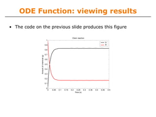
30. ODE Function: viewing results
• To solve and plot the ODEs on the previous slide:
» [t,y]=ode45('chem',[0 0.5],[0 1]);
assumes that only chemical B exists initially
» plot(t,y(:,1),'k','LineWidth',1.5);
» hold on;
» plot(t,y(:,2),'r','LineWidth',1.5);
» legend('A','B');
» xlabel('Time (s)');
» ylabel('Amount of chemical (g)');
» title('Chem reaction');

31. ODE Function: viewing results
• The code on the previous slide produces this figure
Chem reaction
1
A
0.9 B
0.8
0.7
Amount of chemical (g)
0.6
0.5
0.4
0.3
0.2
0.1
0
0 0.05 0.1 0.15 0.2 0.25 0.3 0.35 0.4 0.45 0.5
Time (s)

32. Higher Order Equations
• Must make into a system of first-order equations to use
ODE solvers
• Nonlinear is OK!
• Pendulum example:
g
&&
θ+ sin (θ ) = 0
L
g
&&
θ =− sin (θ )
L
&
let θ = γ
g
γ& = − sin (θ )
L
v ⎡θ ⎤
x=⎢ ⎥
⎣γ ⎦
v &
dx ⎡θ ⎤
=⎢ ⎥
dt ⎣γ& ⎦
Courtesy of The MathWorks, Inc. Used with permission.

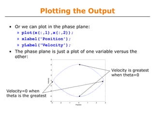
33. Plotting the Output
• We can solve for the position and velocity of the pendulum:
» [t,x]=ode45('pendulum',[0 10],[0.9*pi 0]);
assume pendulum is almost vertical (at top)
» plot(t,x(:,1));
» hold on;
» plot(t,x(:,2),'r');
» legend('Position','Velocity');
8
Position
Velocity
6
Velocity (m/s)
Position in terms of 4
angle (rad) 2
0
-2
-4
-6
-8
0 1 2 3 4 5 6 7 8 9 10

34. Plotting the Output
• Or we can plot in the phase plane:
» plot(x(:,1),x(:,2));
» xlabel('Position');
» yLabel('Velocity');
• The phase plane is just a plot of one variable versus the
other: 8
6
4
Velocity is greatest
2 when theta=0
Velocity
0
-2
Velocity=0 when -4
theta is the greatest -6
-8
-3 -2 -1 0 1 2 3
Position

35. ODE Solvers: Custom Options
• MATLAB's ODE solvers use a variable timestep
• Sometimes a fixed timestep is desirable
» [t,y]=ode45('chem',[0:0.001:0.5],[0 1]);
Specify the timestep by giving a vector of times
The function will be evaluated at the specified points
Fixed timestep is usually slower (if timestep is small) and
possibly inaccurate (if timestep is too large)
• You can customize the error tolerances using odeset
» options=odeset('RelTol',1e-6,'AbsTol',1e-10);
» [t,y]=ode45('chem',[0 0.5],[0 1],options);
This guarantees that the error at each step is less than
RelTol times the value at that step, and less than AbsTol
Decreasing error tolerance can considerably slow the solver
See doc odeset for a list of options you can customize

36. Exercise: ODE
• Use ODE45 to solve this differential equation on the range
t=[0 10], with initial condition y(0) = 10: dy/dt=-t*y/10.
Plot the result.

37. Exercise: ODE
• Use ODE45 to solve this differential equation on the range
t=[0 10], with initial condition y(0) = 10: dy/dt=-t*y/10.
Plot the result.
» function dydt=odefun(t,y)
» dydt=-t*y/10;
» [t,y]=ode45(‘odefun’,[0 10],10);
» plot(t,y);

38. End of Lecture 3
(1) Linear Algebra
(2) Polynomials
(3) Optimization
(4) Differentiation/Integration
(5) Differential Equations
We're almost done!

39. Issues with ODEs
• Stability and accuracy
if step size is too large, solutions might blow up
if step size is too small, requires a long time to solve
use odeset to control errors
– decrease error tolerances to get more accurate
results
– increase error tolerances to speed up computation
(beware of instability!)
• Main thing to remember about ODEs
Pick the most appropriate solver for your problem
If ode45 is taking too long, try ode15s