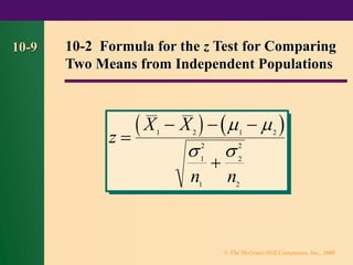
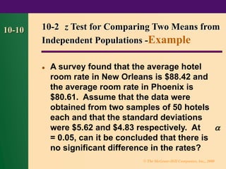
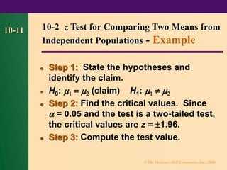
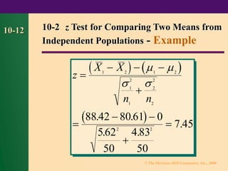
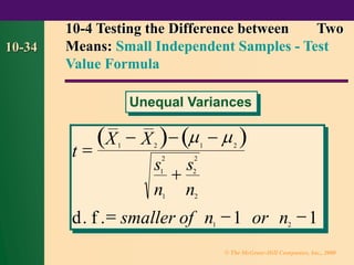
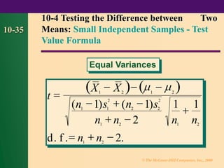
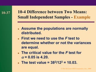
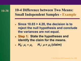
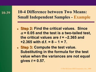
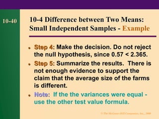
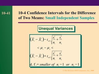
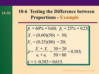
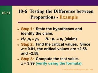
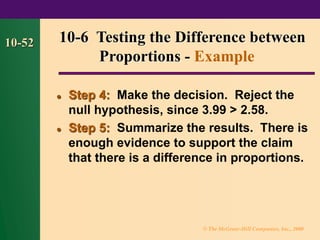
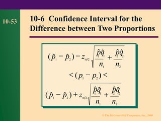
© The McGraw-Hill Companies, Inc., 2000
10-1
Chapter 10
Testing the Difference between
Means, Variances, and
Proportions
© The McGraw-Hill Companies, Inc., 2000
10-2
Outline
⚫ 10-1 Introduction
⚫ 10-2 Testing the Difference
between Two Means: Large
Samples
⚫ 10-3 Testing the Difference
between Two Variances
© The McGraw-Hill Companies, Inc., 2000
10-3
Outline
⚫ 10-4 Testing the Difference
between Two Means: Small
Independent Samples
⚫ 10-5 Testing the Difference
between Two Means: Small
Dependent Samples
© The McGraw-Hill Companies, Inc., 2000
10-4
Outline
⚫ 10-6 Testing the Difference
between Proportions
© The McGraw-Hill Companies, Inc., 2000
10-5
Objectives
⚫ Test the difference between two
large sample means using the z test.
⚫ Test the difference between two
variances or standard deviations.
⚫ Test the difference between two
means for small independent
samples.
© The McGraw-Hill Companies, Inc., 2000
10-6
Objectives
⚫ Test the difference between two
means for small dependent
samples.
⚫ Test the difference between two
proportions.
© The McGraw-Hill Companies, Inc., 2000
10-7 10-2 Testing the Difference between
Two Means: Large Samples
⚫ Assumptions for this test:
⚫ Samples are independent.
⚫ The sampling populations must
be normally distributed.
⚫ Standard deviations are known
or samples must be at least 30.
© The McGraw-Hill Companies, Inc., 2000
10-8 10-2 Testing the Difference between
Two Means: Large Samples
 
1
2
, 1
n s
2
2
, 2
n s
1
2
, 1
 
2
2
, 2
© The McGraw-Hill Companies, Inc., 2000
10-9 10-2 Formula for the z Test for Comparing
Two Means from Independent Populations
( ) ( )
z
X X
n n
=
− − −
+
1 2 1 2
1
2
1
2
2
2
 
 
© The McGraw-Hill Companies, Inc., 2000
10-10 10-2 z Test for Comparing Two Means from
Independent Populations -Example
⚫ A survey found that the average hotel
room rate in New Orleans is $88.42 and
the average room rate in Phoenix is
$80.61. Assume that the data were
obtained from two samples of 50 hotels
each and that the standard deviations
were $5.62 and $4.83 respectively. At 
= 0.05, can it be concluded that there is
no significant difference in the rates?
© The McGraw-Hill Companies, Inc., 2000
10-11
⚫ Step 1: State the hypotheses and
identify the claim.
⚫ H0:  =  (claim) H1:   
⚫ Step 2: Find the critical values. Since
 = 0.05 and the test is a two-tailed test,
the critical values are z = 1.96.
⚫ Step 3: Compute the test value.
10-2 z Test for Comparing Two Means from
Independent Populations - Example
© The McGraw-Hill Companies, Inc., 2000
10-12 10-2 z Test for Comparing Two Means from
Independent Populations - Example
( ) ( )
( )
z
X X
n n
=
− − −
+
=
− −
+
=
1 2 1 2
1
2
1
2
2
2
2 2
88 42 80 61 0
562
50
4 83
50
7 45
 
 
. .
. .
.
© The McGraw-Hill Companies, Inc., 2000
10-13
⚫ Step 4: Make the decision. Reject the
null hypothesis at  = 0.05, since
7.45 > 1.96.
⚫ Step 5: Summarize the results. There is
enough evidence to reject the claim that
the means are equal. Hence, there is a
significant difference in the rates.
10-2 z Test for Comparing Two Means from
Independent Populations - Example
© The McGraw-Hill Companies, Inc., 2000
10-14
10-2 P-Values
⚫ The P-values for the tests can be
determined using the same procedure
as shown in Section 9-3.
⚫ The P-value for the previous example
will be: P-value = 2P(z > 7.45)  2(0) = 0.
⚫ You will reject the null hypothesis since
the P-value = 0 <  = 0.05.
© The McGraw-Hill Companies, Inc., 2000
10-15
10-2 Formula for Confidence Interval for
Difference Between Two Means : Large
Samples
( )
( )
X X
n n
X X
n n
1 2
1
2
1
2
2
2
1 2
1 2
1
2
1
2
2
2
− − +
 − 
− + +
 
 
 
z 2
 )
(
z 2
 )
(
© The McGraw-Hill Companies, Inc., 2000
10-16 10-2 Confidence Interval for Difference of Two
Means: Large Samples - Example
⚫ Find the 95% confidence interval for the
difference between the means for the
data in the previous example.
⚫ Substituting in the formula one gets
(verify) 5.76 <  −  < 9.86.
⚫ Since the confidence interval does not
contain zero, one would reject the null
hypothesis in the previous example.
© The McGraw-Hill Companies, Inc., 2000
10-17 10-3 Testing the Difference Between
Two Variances
⚫ For the comparison of two
variances or standard deviations,
an F test is used.
⚫ The sampling distribution of the
variances is called the
F distribution.
© The McGraw-Hill Companies, Inc., 2000
10-18 10-3 Characteristics of the
F Distribution
⚫ The values of F cannot be negative.
⚫ The distribution is positively skewed.
⚫ The mean value of F is approximately
equal to 1.
⚫ The F distribution is a family of curves
based on the degrees of freedom of the
variance of the numerator and
denominator.
© The McGraw-Hill Companies, Inc., 2000
10-19
10-3 Curves for the F Distribution
0
1.0
0.0
0
1.0
0.0
© The McGraw-Hill Companies, Inc., 2000
10-20
10-3 Formula for the F Test
.
F
s
s
where s is the larger of the two
numerator of freedom n
denominator of freedom n
n is the sample size from which the larger
was obtained
=
= −
= −
1
2
2
2
1
2
1
2
1
1
1
variances
degrees
degrees
variance
.
© The McGraw-Hill Companies, Inc., 2000
10-21
⚫ The populations from which the
samples were obtained must be
normally distributed.
⚫ The samples must be independent
of each other.
10-3 Assumptions for Testing the
Difference between Two Variances
© The McGraw-Hill Companies, Inc., 2000
10-22
⚫ A researcher wishes to see whether the
variances of the heart rates (in beats per
minute) of smokers are different from
the variances of heart rates of people
who do not smoke. Two samples are
selected, and the data are given on the
next slide. Using  = 0.05, is there
enough evidence to support the claim?
10-3 Testing the Difference between
Two Variances - Example
© The McGraw-Hill Companies, Inc., 2000
10-23
⚫ For smokers n1 = 26 and = 36; for
nonsmokers n2 = 18 and = 10.
⚫ Step 1: State the hypotheses and
identify the claim.
H0: = H1:  (claim)
10-3 Testing the Difference between
Two Variances - Example
s
1
1
s
2
2
2
1 2
2 2
1
2
2
© The McGraw-Hill Companies, Inc., 2000
10-24
⚫ Step 2: Find the critical value. Since
 = 0.05 and the test is a two-tailed test,
use the 0.025 table. Here d.f. N. = 26 – 1
= 25, and d.f.D. = 18 – 1 = 17. The
critical value is F = 2.56.
⚫ Step 3: Compute the test value.
F = / = 36/10 = 3.6.
10-3 Testing the Difference between
Two Variances - Example
s
2
2
s
2
1
© The McGraw-Hill Companies, Inc., 2000
10-25
⚫ Step 4: Make the decision. Reject the
null hypothesis, since 3.6 > 2.56.
⚫ Step 5: Summarize the results. There is
enough evidence to support the claim
that the variances are different.
10-3 Testing the Difference between
Two Variances - Example
© The McGraw-Hill Companies, Inc., 2000
10-26 10-3 Testing the Difference between
Two Variances - Example


© The McGraw-Hill Companies, Inc., 2000
10-27
⚫ An instructor hypothesizes that the
standard deviation of the final exam
grades in her statistics class is larger
for the male students than it is for the
female students. The data from the final
exam for the last semester are: males
n1 = 16 and s1 = 4.2; females n2 = 18 and
s2 = 2.3.
10-3 Testing the Difference between
Two Variances - Example
© The McGraw-Hill Companies, Inc., 2000
10-28
⚫ Is there enough evidence to support her
claim, using  = 0.01?
⚫ Step 1: State the hypotheses and
identify the claim.
H0:  H1:  (claim)
10-3 Testing the Difference between
Two Variances - Example
2
1 2
2 2
1 2
2
© The McGraw-Hill Companies, Inc., 2000
10-29
⚫ Step 2: Find the critical value. Here,
d.f.N. = 16 –1 = 15, and
d.f.D. = 18 –1 = 17.
For  = 0.01 table, the critical value is
F = 3.31.
⚫ Step 3: Compute the test value.
F = (4.2)2/(2.3)2 = 3.33.
10-3 Testing the Difference between
Two Variances - Example
© The McGraw-Hill Companies, Inc., 2000
10-30
⚫ Step 4: Make the decision. Reject the
null hypothesis, since 3.33 > 3.31.
⚫ Step 5: Summarize the results. There is
enough evidence to support the claim
that the standard deviation of the final
exam grades for the male students is
larger than that for the female students.
10-3 Testing the Difference between
Two Variances - Example
© The McGraw-Hill Companies, Inc., 2000
10-31 10-3 Testing the Difference between
Two Variances - Example


© The McGraw-Hill Companies, Inc., 2000
10-32
⚫ When the sample sizes are small (< 30)
and the population variances are
unknown, a t test is used to test the
difference between means.
⚫ The two samples are assumed to be
independent and the sampling
populations are normally or
approximately normally distributed.
10-4 Testing the Difference between
Two Means: Small Independent Samples
© The McGraw-Hill Companies, Inc., 2000
10-33
⚫ There are two options for the use of the
t test.
⚫ When the variances of the populations
are equal and when they are not equal.
⚫ The F test can be used to establish
whether the variances are equal or not.
10-4 Testing the Difference between
Two Means: Small Independent Samples
© The McGraw-Hill Companies, Inc., 2000
10-34
( ) ( )
t
X X
s
n
s
n
d f smaller of n or n
=
− − −
+
= − −
1 2 1 2
1
2
1
2
2
2
1 2
1 1
 
. .
10-4 Testing the Difference between Two
Means: Small Independent Samples - Test
Value Formula
Unequal Variances
© The McGraw-Hill Companies, Inc., 2000
10-35
10-4 Testing the Difference between Two
Means: Small Independent Samples - Test
Value Formula
Equal Variances
( ) ( )
t
X X
n s n s
n n n n
d f n n
=
− − −
− + −
+ −
+
= + −
1 2 1 2
1 1
2
2 2
2
1 2 1 2
1 2
1 1
2
1 1
2
 
( ) ( )
. . .
© The McGraw-Hill Companies, Inc., 2000
10-36
⚫ The average size of a farm in Greene County,
PA, is 199 acres, and the average size of a farm
in Indiana County, PA, is 191 acres. Assume
the data were obtained from two samples with
standard deviations of 12 acres and 38 acres,
respectively, and the sample sizes are 10 farms
from Greene County and 8 farms in Indiana
County. Can it be concluded at  = 0.05 that
the average size of the farms in the two
counties is different?
10-4 Difference between Two Means:
Small Independent Samples - Example
© The McGraw-Hill Companies, Inc., 2000
10-37
⚫ Assume the populations are normally
distributed.
⚫ First we need to use the F test to
determine whether or not the variances
are equal.
⚫ The critical value for the F test for
 = 0.05 is 4.20.
⚫ The test value = 382/122 = 10.03.
10-4 Difference between Two Means:
Small Independent Samples - Example
© The McGraw-Hill Companies, Inc., 2000
10-38
⚫ Since 10.03 > 4.20, the decision is to
reject the null hypothesis and conclude
the variances are not equal.
⚫ Step 1: State the hypotheses and
identify the claim for the means.
⚫ H0:  =  H1:    (claim)
10-4 Difference between Two Means:
Small Independent Samples - Example
© The McGraw-Hill Companies, Inc., 2000
10-39
⚫ Step 2: Find the critical values. Since
 = 0.05 and the test is a two-tailed test,
the critical values are t = –2.365 and
+2.365 with d.f. = 8 – 1 = 7.
⚫ Step 3: Compute the test value.
Substituting in the formula for the test
value when the variances are not equal
gives t = 0.57.
10-4 Difference between Two Means:
Small Independent Samples - Example
© The McGraw-Hill Companies, Inc., 2000
10-40
⚫ Step 4: Make the decision. Do not reject
the null hypothesis, since 0.57 < 2.365.
⚫ Step 5: Summarize the results. There is
not enough evidence to support the
claim that the average size of the farms
is different.
⚫ Note: If the the variances were equal -
use the other test value formula.
10-4 Difference between Two Means:
Small Independent Samples - Example
© The McGraw-Hill Companies, Inc., 2000
10-41
( )
( )
X X t
X X t
d f smaller of n or n
1 2 2
1 2
1 2 2
1 2
1 1
− −
s
n
s
n
1
2
1
2
2
2
+
− 
− +
= − −


 
<
. .
10-4 Confidence Intervals for the Difference
of Two Means: Small Independent Samples
Unequal Variances
s
n
s
n
1
2
1
2
2
2
+
© The McGraw-Hill Companies, Inc., 2000
10-42
( )
( )
X X
n s n s
n n − 2 n n
X X
n s n s
n n − 2 n n
d f n n
1 2
1 1
2
2 2
2
1 2 1 2
1 2
1 2
1 1
2
2 2
2
1 2 1 2
1 2
1 1 1 1
1 1 1 1
2
− −
− + −
+
+
− 
− +
− + −
+
+
= + −
t 2

t 2

 
( ) ( )
( ) ( )
. . .
<
10-4 Confidence Intervals for the Difference
of Two Means: Small Independent Samples
Equal Variances


© The McGraw-Hill Companies, Inc., 2000
10-43
⚫ When the values are dependent,
employ a t test on the differences.
⚫ Denote the differences with the
symbol D, the mean of the population
of differences with D, and the sample
standard deviation of the differences
with sD.
10-5 Testing the Difference between
Two Means: Small Dependent Samples
© The McGraw-Hill Companies, Inc., 2000
10-44
t
D
s n
where
D sample mean
of freedom n
D
D
=
−
=
= −

degrees 1
10-5 Testing the Difference between Two
Means: Small Dependent Samples -
Formula for the test value.
© The McGraw-Hill Companies, Inc., 2000
10-45
⚫ Note: This test is similar to a
one sample t test, except it is
done on the differences when
the samples are dependent.
10-5 Testing the Difference between Two
Means: Small Dependent Samples -
Formula for the test value.
© The McGraw-Hill Companies, Inc., 2000
10-46
– +
. .=
D t s n D t s n
d f n
 D D  D
2 2
1
   
−

10-5 Confidence Interval for the Difference
between Two Means: Small Dependent
Samples - Formula.
Note: This formula is similar to the confidence
interval formula for a single population mean
when the population variance is unknown.
© The McGraw-Hill Companies, Inc., 2000
10-47 10-6 Testing the Difference between
Proportions - Formula
; = -
1
2
z
p p p p
pq
n n
where n and n are sample sizes
p
X X
n n
q p p
X
n
p
X
n
X number of successes in sample
=
− − −
+






=
+
+
= =
=
=
(   ) ( )
;  ;  ;
1 2 1 2
1 2
1 2
1 2
1 2
1
1
1
2
2
2
1 1
1
1
2
© The McGraw-Hill Companies, Inc., 2000
10-48
⚫ A sample of 50 randomly selected men
with high triglyceride levels consumed
2 tablespoons of oat bran daily for six
weeks. After six weeks, 60% of the
men had lowered their triglyceride
level. A sample of 80 men consumed 2
tablespoons of wheat bran for six
weeks. (continued on next slide)
10-6 Testing the Difference between
Proportions - Example
© The McGraw-Hill Companies, Inc., 2000
10-49
⚫ After six weeks, 25% had lower
triclyceride levels. Is there significant
differences in the two proportions, at
the 0.01 level of significance?
10-6 Testing the Difference between
Proportions - Example
© The McGraw-Hill Companies, Inc., 2000
10-50
 . ;  . ;
p p
X
p
X X
n n
q
1 2
1
1 2
1 2
60% 0 60 25% 0 25
30 20
50 80
0385
1 0 385 0615
= = = =
+
+
= (0.60)(50) = 30;
X = (0.25)(80) = 20;
= =
+
+
= . ;
= – . = . .
2
10-6 Testing the Difference between
Proportions - Example
© The McGraw-Hill Companies, Inc., 2000
10-51
⚫ Step 1: State the hypotheses and
identify the claim.
⚫ H0: p1 = p2 H1: p1  p2 (claim)
⚫ Step 2: Find the critical values. Since
 = 0.01, the critical values are +2.58
and –2.58.
⚫ Step 3: Compute the test value.
z = 3.99 (verify using the formula).
10-6 Testing the Difference between
Proportions - Example
© The McGraw-Hill Companies, Inc., 2000
10-52
⚫ Step 4: Make the decision. Reject the
null hypothesis, since 3.99 > 2.58.
⚫ Step 5: Summarize the results. There is
enough evidence to support the claim
that there is a difference in proportions.
10-6 Testing the Difference between
Proportions - Example
© The McGraw-Hill Companies, Inc., 2000
10-53 10-6 Confidence Interval for the
Difference between Two Proportions
(   )
( )
(   )
p p z
p p
p p z
1 2 2
1 2
1 2 2
− −
 − 
− +


n n
1
+


pq
1 1


pq
2 2
2
n n
1
+


pq
1 1


pq
2 2
2

bman10.pdf formulas and notes on how to get mean

  • 1.
    © The McGraw-HillCompanies, Inc., 2000 10-1 Chapter 10 Testing the Difference between Means, Variances, and Proportions
  • 2.
    © The McGraw-HillCompanies, Inc., 2000 10-2 Outline ⚫ 10-1 Introduction ⚫ 10-2 Testing the Difference between Two Means: Large Samples ⚫ 10-3 Testing the Difference between Two Variances
  • 3.
    © The McGraw-HillCompanies, Inc., 2000 10-3 Outline ⚫ 10-4 Testing the Difference between Two Means: Small Independent Samples ⚫ 10-5 Testing the Difference between Two Means: Small Dependent Samples
  • 4.
    © The McGraw-HillCompanies, Inc., 2000 10-4 Outline ⚫ 10-6 Testing the Difference between Proportions
  • 5.
    © The McGraw-HillCompanies, Inc., 2000 10-5 Objectives ⚫ Test the difference between two large sample means using the z test. ⚫ Test the difference between two variances or standard deviations. ⚫ Test the difference between two means for small independent samples.
  • 6.
    © The McGraw-HillCompanies, Inc., 2000 10-6 Objectives ⚫ Test the difference between two means for small dependent samples. ⚫ Test the difference between two proportions.
  • 7.
    © The McGraw-HillCompanies, Inc., 2000 10-7 10-2 Testing the Difference between Two Means: Large Samples ⚫ Assumptions for this test: ⚫ Samples are independent. ⚫ The sampling populations must be normally distributed. ⚫ Standard deviations are known or samples must be at least 30.
  • 8.
    © The McGraw-HillCompanies, Inc., 2000 10-8 10-2 Testing the Difference between Two Means: Large Samples   1 2 , 1 n s 2 2 , 2 n s 1 2 , 1   2 2 , 2
  • 9.
    © The McGraw-HillCompanies, Inc., 2000 10-9 10-2 Formula for the z Test for Comparing Two Means from Independent Populations ( ) ( ) z X X n n = − − − + 1 2 1 2 1 2 1 2 2 2    
  • 10.
    © The McGraw-HillCompanies, Inc., 2000 10-10 10-2 z Test for Comparing Two Means from Independent Populations -Example ⚫ A survey found that the average hotel room rate in New Orleans is $88.42 and the average room rate in Phoenix is $80.61. Assume that the data were obtained from two samples of 50 hotels each and that the standard deviations were $5.62 and $4.83 respectively. At  = 0.05, can it be concluded that there is no significant difference in the rates?
  • 11.
    © The McGraw-HillCompanies, Inc., 2000 10-11 ⚫ Step 1: State the hypotheses and identify the claim. ⚫ H0:  =  (claim) H1:    ⚫ Step 2: Find the critical values. Since  = 0.05 and the test is a two-tailed test, the critical values are z = 1.96. ⚫ Step 3: Compute the test value. 10-2 z Test for Comparing Two Means from Independent Populations - Example
  • 12.
    © The McGraw-HillCompanies, Inc., 2000 10-12 10-2 z Test for Comparing Two Means from Independent Populations - Example ( ) ( ) ( ) z X X n n = − − − + = − − + = 1 2 1 2 1 2 1 2 2 2 2 2 88 42 80 61 0 562 50 4 83 50 7 45     . . . . .
  • 13.
    © The McGraw-HillCompanies, Inc., 2000 10-13 ⚫ Step 4: Make the decision. Reject the null hypothesis at  = 0.05, since 7.45 > 1.96. ⚫ Step 5: Summarize the results. There is enough evidence to reject the claim that the means are equal. Hence, there is a significant difference in the rates. 10-2 z Test for Comparing Two Means from Independent Populations - Example
  • 14.
    © The McGraw-HillCompanies, Inc., 2000 10-14 10-2 P-Values ⚫ The P-values for the tests can be determined using the same procedure as shown in Section 9-3. ⚫ The P-value for the previous example will be: P-value = 2P(z > 7.45)  2(0) = 0. ⚫ You will reject the null hypothesis since the P-value = 0 <  = 0.05.
  • 15.
    © The McGraw-HillCompanies, Inc., 2000 10-15 10-2 Formula for Confidence Interval for Difference Between Two Means : Large Samples ( ) ( ) X X n n X X n n 1 2 1 2 1 2 2 2 1 2 1 2 1 2 1 2 2 2 − − +  −  − + +       z 2  ) ( z 2  ) (
  • 16.
    © The McGraw-HillCompanies, Inc., 2000 10-16 10-2 Confidence Interval for Difference of Two Means: Large Samples - Example ⚫ Find the 95% confidence interval for the difference between the means for the data in the previous example. ⚫ Substituting in the formula one gets (verify) 5.76 <  −  < 9.86. ⚫ Since the confidence interval does not contain zero, one would reject the null hypothesis in the previous example.
  • 17.
    © The McGraw-HillCompanies, Inc., 2000 10-17 10-3 Testing the Difference Between Two Variances ⚫ For the comparison of two variances or standard deviations, an F test is used. ⚫ The sampling distribution of the variances is called the F distribution.
  • 18.
    © The McGraw-HillCompanies, Inc., 2000 10-18 10-3 Characteristics of the F Distribution ⚫ The values of F cannot be negative. ⚫ The distribution is positively skewed. ⚫ The mean value of F is approximately equal to 1. ⚫ The F distribution is a family of curves based on the degrees of freedom of the variance of the numerator and denominator.
  • 19.
    © The McGraw-HillCompanies, Inc., 2000 10-19 10-3 Curves for the F Distribution 0 1.0 0.0 0 1.0 0.0
  • 20.
    © The McGraw-HillCompanies, Inc., 2000 10-20 10-3 Formula for the F Test . F s s where s is the larger of the two numerator of freedom n denominator of freedom n n is the sample size from which the larger was obtained = = − = − 1 2 2 2 1 2 1 2 1 1 1 variances degrees degrees variance .
  • 21.
    © The McGraw-HillCompanies, Inc., 2000 10-21 ⚫ The populations from which the samples were obtained must be normally distributed. ⚫ The samples must be independent of each other. 10-3 Assumptions for Testing the Difference between Two Variances
  • 22.
    © The McGraw-HillCompanies, Inc., 2000 10-22 ⚫ A researcher wishes to see whether the variances of the heart rates (in beats per minute) of smokers are different from the variances of heart rates of people who do not smoke. Two samples are selected, and the data are given on the next slide. Using  = 0.05, is there enough evidence to support the claim? 10-3 Testing the Difference between Two Variances - Example
  • 23.
    © The McGraw-HillCompanies, Inc., 2000 10-23 ⚫ For smokers n1 = 26 and = 36; for nonsmokers n2 = 18 and = 10. ⚫ Step 1: State the hypotheses and identify the claim. H0: = H1:  (claim) 10-3 Testing the Difference between Two Variances - Example s 1 1 s 2 2 2 1 2 2 2 1 2 2
  • 24.
    © The McGraw-HillCompanies, Inc., 2000 10-24 ⚫ Step 2: Find the critical value. Since  = 0.05 and the test is a two-tailed test, use the 0.025 table. Here d.f. N. = 26 – 1 = 25, and d.f.D. = 18 – 1 = 17. The critical value is F = 2.56. ⚫ Step 3: Compute the test value. F = / = 36/10 = 3.6. 10-3 Testing the Difference between Two Variances - Example s 2 2 s 2 1
  • 25.
    © The McGraw-HillCompanies, Inc., 2000 10-25 ⚫ Step 4: Make the decision. Reject the null hypothesis, since 3.6 > 2.56. ⚫ Step 5: Summarize the results. There is enough evidence to support the claim that the variances are different. 10-3 Testing the Difference between Two Variances - Example
  • 26.
    © The McGraw-HillCompanies, Inc., 2000 10-26 10-3 Testing the Difference between Two Variances - Example  
  • 27.
    © The McGraw-HillCompanies, Inc., 2000 10-27 ⚫ An instructor hypothesizes that the standard deviation of the final exam grades in her statistics class is larger for the male students than it is for the female students. The data from the final exam for the last semester are: males n1 = 16 and s1 = 4.2; females n2 = 18 and s2 = 2.3. 10-3 Testing the Difference between Two Variances - Example
  • 28.
    © The McGraw-HillCompanies, Inc., 2000 10-28 ⚫ Is there enough evidence to support her claim, using  = 0.01? ⚫ Step 1: State the hypotheses and identify the claim. H0:  H1:  (claim) 10-3 Testing the Difference between Two Variances - Example 2 1 2 2 2 1 2 2
  • 29.
    © The McGraw-HillCompanies, Inc., 2000 10-29 ⚫ Step 2: Find the critical value. Here, d.f.N. = 16 –1 = 15, and d.f.D. = 18 –1 = 17. For  = 0.01 table, the critical value is F = 3.31. ⚫ Step 3: Compute the test value. F = (4.2)2/(2.3)2 = 3.33. 10-3 Testing the Difference between Two Variances - Example
  • 30.
    © The McGraw-HillCompanies, Inc., 2000 10-30 ⚫ Step 4: Make the decision. Reject the null hypothesis, since 3.33 > 3.31. ⚫ Step 5: Summarize the results. There is enough evidence to support the claim that the standard deviation of the final exam grades for the male students is larger than that for the female students. 10-3 Testing the Difference between Two Variances - Example
  • 31.
    © The McGraw-HillCompanies, Inc., 2000 10-31 10-3 Testing the Difference between Two Variances - Example  
  • 32.
    © The McGraw-HillCompanies, Inc., 2000 10-32 ⚫ When the sample sizes are small (< 30) and the population variances are unknown, a t test is used to test the difference between means. ⚫ The two samples are assumed to be independent and the sampling populations are normally or approximately normally distributed. 10-4 Testing the Difference between Two Means: Small Independent Samples
  • 33.
    © The McGraw-HillCompanies, Inc., 2000 10-33 ⚫ There are two options for the use of the t test. ⚫ When the variances of the populations are equal and when they are not equal. ⚫ The F test can be used to establish whether the variances are equal or not. 10-4 Testing the Difference between Two Means: Small Independent Samples
  • 34.
    © The McGraw-HillCompanies, Inc., 2000 10-34 ( ) ( ) t X X s n s n d f smaller of n or n = − − − + = − − 1 2 1 2 1 2 1 2 2 2 1 2 1 1   . . 10-4 Testing the Difference between Two Means: Small Independent Samples - Test Value Formula Unequal Variances
  • 35.
    © The McGraw-HillCompanies, Inc., 2000 10-35 10-4 Testing the Difference between Two Means: Small Independent Samples - Test Value Formula Equal Variances ( ) ( ) t X X n s n s n n n n d f n n = − − − − + − + − + = + − 1 2 1 2 1 1 2 2 2 2 1 2 1 2 1 2 1 1 2 1 1 2   ( ) ( ) . . .
  • 36.
    © The McGraw-HillCompanies, Inc., 2000 10-36 ⚫ The average size of a farm in Greene County, PA, is 199 acres, and the average size of a farm in Indiana County, PA, is 191 acres. Assume the data were obtained from two samples with standard deviations of 12 acres and 38 acres, respectively, and the sample sizes are 10 farms from Greene County and 8 farms in Indiana County. Can it be concluded at  = 0.05 that the average size of the farms in the two counties is different? 10-4 Difference between Two Means: Small Independent Samples - Example
  • 37.
    © The McGraw-HillCompanies, Inc., 2000 10-37 ⚫ Assume the populations are normally distributed. ⚫ First we need to use the F test to determine whether or not the variances are equal. ⚫ The critical value for the F test for  = 0.05 is 4.20. ⚫ The test value = 382/122 = 10.03. 10-4 Difference between Two Means: Small Independent Samples - Example
  • 38.
    © The McGraw-HillCompanies, Inc., 2000 10-38 ⚫ Since 10.03 > 4.20, the decision is to reject the null hypothesis and conclude the variances are not equal. ⚫ Step 1: State the hypotheses and identify the claim for the means. ⚫ H0:  =  H1:    (claim) 10-4 Difference between Two Means: Small Independent Samples - Example
  • 39.
    © The McGraw-HillCompanies, Inc., 2000 10-39 ⚫ Step 2: Find the critical values. Since  = 0.05 and the test is a two-tailed test, the critical values are t = –2.365 and +2.365 with d.f. = 8 – 1 = 7. ⚫ Step 3: Compute the test value. Substituting in the formula for the test value when the variances are not equal gives t = 0.57. 10-4 Difference between Two Means: Small Independent Samples - Example
  • 40.
    © The McGraw-HillCompanies, Inc., 2000 10-40 ⚫ Step 4: Make the decision. Do not reject the null hypothesis, since 0.57 < 2.365. ⚫ Step 5: Summarize the results. There is not enough evidence to support the claim that the average size of the farms is different. ⚫ Note: If the the variances were equal - use the other test value formula. 10-4 Difference between Two Means: Small Independent Samples - Example
  • 41.
    © The McGraw-HillCompanies, Inc., 2000 10-41 ( ) ( ) X X t X X t d f smaller of n or n 1 2 2 1 2 1 2 2 1 2 1 1 − − s n s n 1 2 1 2 2 2 + −  − + = − −     < . . 10-4 Confidence Intervals for the Difference of Two Means: Small Independent Samples Unequal Variances s n s n 1 2 1 2 2 2 +
  • 42.
    © The McGraw-HillCompanies, Inc., 2000 10-42 ( ) ( ) X X n s n s n n − 2 n n X X n s n s n n − 2 n n d f n n 1 2 1 1 2 2 2 2 1 2 1 2 1 2 1 2 1 1 2 2 2 2 1 2 1 2 1 2 1 1 1 1 1 1 1 1 2 − − − + − + + −  − + − + − + + = + − t 2  t 2    ( ) ( ) ( ) ( ) . . . < 10-4 Confidence Intervals for the Difference of Two Means: Small Independent Samples Equal Variances  
  • 43.
    © The McGraw-HillCompanies, Inc., 2000 10-43 ⚫ When the values are dependent, employ a t test on the differences. ⚫ Denote the differences with the symbol D, the mean of the population of differences with D, and the sample standard deviation of the differences with sD. 10-5 Testing the Difference between Two Means: Small Dependent Samples
  • 44.
    © The McGraw-HillCompanies, Inc., 2000 10-44 t D s n where D sample mean of freedom n D D = − = = −  degrees 1 10-5 Testing the Difference between Two Means: Small Dependent Samples - Formula for the test value.
  • 45.
    © The McGraw-HillCompanies, Inc., 2000 10-45 ⚫ Note: This test is similar to a one sample t test, except it is done on the differences when the samples are dependent. 10-5 Testing the Difference between Two Means: Small Dependent Samples - Formula for the test value.
  • 46.
    © The McGraw-HillCompanies, Inc., 2000 10-46 – + . .= D t s n D t s n d f n  D D  D 2 2 1     −  10-5 Confidence Interval for the Difference between Two Means: Small Dependent Samples - Formula. Note: This formula is similar to the confidence interval formula for a single population mean when the population variance is unknown.
  • 47.
    © The McGraw-HillCompanies, Inc., 2000 10-47 10-6 Testing the Difference between Proportions - Formula ; = - 1 2 z p p p p pq n n where n and n are sample sizes p X X n n q p p X n p X n X number of successes in sample X number of successes in sample = − − − +       = + + = = = = (   ) ( ) ;  ;  ; 1 2 1 2 1 2 1 2 1 2 1 2 1 1 1 2 2 2 1 1 1 1 2
  • 48.
    © The McGraw-HillCompanies, Inc., 2000 10-48 ⚫ A sample of 50 randomly selected men with high triglyceride levels consumed 2 tablespoons of oat bran daily for six weeks. After six weeks, 60% of the men had lowered their triglyceride level. A sample of 80 men consumed 2 tablespoons of wheat bran for six weeks. (continued on next slide) 10-6 Testing the Difference between Proportions - Example
  • 49.
    © The McGraw-HillCompanies, Inc., 2000 10-49 ⚫ After six weeks, 25% had lower triclyceride levels. Is there significant differences in the two proportions, at the 0.01 level of significance? 10-6 Testing the Difference between Proportions - Example
  • 50.
    © The McGraw-HillCompanies, Inc., 2000 10-50  . ;  . ; p p X p X X n n q 1 2 1 1 2 1 2 60% 0 60 25% 0 25 30 20 50 80 0385 1 0 385 0615 = = = = + + = (0.60)(50) = 30; X = (0.25)(80) = 20; = = + + = . ; = – . = . . 2 10-6 Testing the Difference between Proportions - Example
  • 51.
    © The McGraw-HillCompanies, Inc., 2000 10-51 ⚫ Step 1: State the hypotheses and identify the claim. ⚫ H0: p1 = p2 H1: p1  p2 (claim) ⚫ Step 2: Find the critical values. Since  = 0.01, the critical values are +2.58 and –2.58. ⚫ Step 3: Compute the test value. z = 3.99 (verify using the formula). 10-6 Testing the Difference between Proportions - Example
  • 52.
    © The McGraw-HillCompanies, Inc., 2000 10-52 ⚫ Step 4: Make the decision. Reject the null hypothesis, since 3.99 > 2.58. ⚫ Step 5: Summarize the results. There is enough evidence to support the claim that there is a difference in proportions. 10-6 Testing the Difference between Proportions - Example
  • 53.
    © The McGraw-HillCompanies, Inc., 2000 10-53 10-6 Confidence Interval for the Difference between Two Proportions (   ) ( ) (   ) p p z p p p p z 1 2 2 1 2 1 2 2 − −  −  − +   n n 1 +   pq 1 1   pq 2 2 2 n n 1 +   pq 1 1   pq 2 2 2