Categorical data analysis full lecture note PPT.pptx

Categorical Data Analysis
Stat3062
MINILIK D.
MSc in Biostatistics
Email: minilikderse@gmail.com/minder@dtu.edu.et
Department of Statistics, DTU
31 January 2024

CHAPTER ONE
Introduction about categorical data analysis

A categorical variable is a random variable that can only take finite or countable
many values (categories) .
Categorical variables are variables that can take on one of a limited, and usually
fixed, number of possible values.
variable
Quantitative
variables
Qualitative
variables
Interval
Ratio
Nominal
Ordinal
Count outcome
Categorical analysis

• 1
Response Predictors Methods
Continuous
Nominal/Ordinal, >2 categories ANOVA
Nominal & some continuous ANCOA
Categorical & continuous Multiple Regression
Binary Categorical & continuous Logistic regression
Nominal >2 categories Categorical & continuous Multi-nominal logistic regression
Ordinal Categorical & continuous Ordinal logistic regression
Count
Categorical Log-linear models
Categorical & continuous Poisson regression

The Binomial Distribution
 A binomial distribution is one of the most frequently used a discrete distribution
which is very useful in many practical situations involving two types of outcomes.
 It is the generalization of Bernoulli trial which with only two mutually exclusive and
exhaustive outcomes which are labeled as "success" and "failure".
 Under the assumption of independent and identical trials, Y has the
binomial distribution with the number of trials n and probability of
success π, Y ~Bin(n, π). Therefore, the probability of y successes out of
the n trials is:
 𝑃 𝑌 = 𝑦 =
𝑛!
𝑦!(𝑛−𝑦)!
π𝑦(1 − π)𝑛−𝑦 , y= 0, 1, 2,. . . , n
 E(y) = µ= nπ, and variance of Y (σ2) = nπ (1-π)
 The binomial distribution is always symmetric when π = 0:50. For fixed n,
it becomes more skewed as π moves toward 0 or 1.

 For fixed π, it becomes more symmetric as n increases. When n is large, it can
be approximated by a normal distribution with µ=nπ and σ2= nπ (1 –π).
 Binomial (n, π) can be approx. by Normal (n π; n π (1-nπ)) when n is large (nπ >
5 and n (1- π) > 5).
 R –CODE
dbinom(x,n,p)
dbinom(0:8,8, 0.2)
plot(0:8, dbinom(0:8, 8, .2), type = "h", xlab = "y", ylab = "P(y)")
dbinom(0:25,25, 0.5)
plot(0:25, dbinom(0:25, 25, .5), type = "h", xlab = "y", ylab = "P(y))

The Multinomial Distribution
The multinomial distribution is an extension of binomial distribution. In this case,
each trial has more than two mutually exclusive and exhaustive outcomes.
π𝑖 = P(category i), for each trial, 𝑖=1
𝑐
π𝑖 =1 , where, each trials are independent
Yi = number of trials fall in category i out of n trials
The joint distribution of (Y1,Y2, , , , Y𝑐) has a multinomial distribution, with
probability function
P(Y1= y1, Y2= y2, , , , Y𝑐= y𝑐) =
𝑛!
𝑦1! 𝑦2! …𝑦𝑐!
π1
y1. π2
y2…π𝑐
y𝑐
Where 0≤ yi ≤
n, and 𝑖=1
𝑐
y𝑖 =n
Outcomes Categories
1 2 . . . j total
Observed
Frequency
𝑛1 𝑛2 𝑛𝑗 n
Probability 𝜋1 𝜋2 . . . 𝜋𝑗 1

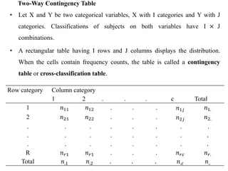
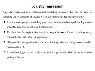
Example 1.4: Suppose proportions of individuals with genotypes AA, Aa, and aa in
a large population are (πAA , πAa, πaa) = (0.25, 0.5, 0.25): Randomly sample n = 5
individuals from the population. The chance of getting 2 AA’s, 2 Aa’s, and 1 aa is
R code
dmultinom(Y=c(y1,y2, , , , y𝑐), prob = c(π1,π2…,π𝑐))
dmultinom(x=c(2,2,1),prob = c(0.25,0.5,0.25))
[1] 0.1171875
dmultinom(x=c(0,3,2), prob = c(0.25,0.5,0.25))
[1] 0.078125
• If (Y1,Y2, , , , Y𝑐) has a multinomial distribution with n trials and category
probabilities (π1,π2…,π𝑐) then
E(Y𝑖) = nπ𝑐, for i= 1.2…..c
Var (Y𝑖) = n π (1 − nπ
Cov(Y𝑖, Y𝑗) = -π𝑖π𝑗

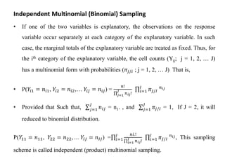
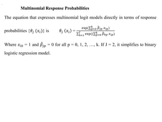
The Poisson distribution
• Poisson distribution is a discrete probability distribution, which is useful for
modeling the number of successes in a certain time, space.
Example 1.5: In a small city, 10 accidents took place in a time of 50 days. Find the
probability that there will be a) two accidents in a day and b) three or more
accidents in a day.
Solution: There are 0.2 accidents per day. Let X be the random variable, the number
of accidents per day
X ～poiss (𝜆 = 0.2) X = 0, 1, 2, ….
𝑃 (𝑋 = 2) =
(0.2)2𝑒−0.2
2!
= 0.0164
b) P (X ≥ 3) = P(X = 3) + P(X = 4) + P(X = 5) +...
= 1- [P(X = 0) + P(X = 1) + P(X = 2)] . . . . . . since
= 1- [0.8187 + 0.1637 + 0.0164] = 0.0012

Statistical inference for a proportion
Most of the time there are two known types of proportion. Such as:
Incidence proportion: proportion at risk that develop a condition over a specified
period of time which is the average risk of events.
Prevalence proportion: proportion with the characteristic or condition at a
particular time.
Statistical inference
Hypothesis testing Confidence interval
One test
Two test
ANOVA

The 100(1-α) % confidence interval for the population proportion π, is given
that
𝜋 ± margin of error = 𝜋 ±z*
π (1−π
𝑛
Testing a Proportion
The sampling distribution for 𝜋 is approximately normal for large sample sizes and
its shape depends solely on for 𝜋 and n. Thus, we can easily test the null
hypothesis:
H0: π = π0 (a given value we are testing).
If H0 is true, the sampling distribution is known
zcal =
𝜋−π0
π (1−π
𝑛
This is valid when both expected counts of successes n π and expected counts of
failures
n(1 − π0) are each greater 5.

Example 1.6: Of 1464 HIV/AIDS patients under HAART treatment in DEBRE
Tabor referral Hospital from 2015-2020, 331 defaulted, while 1113 were
active. Did the proportion of defaulter patients different from one fourth?
Let π denote the proportion of defaulter patients. The hypothesis to be tested is
H0: π0= 0:25 vs H1 π0= 0:25.
The sample proportion of defaulters is π ̂= 331/1614 = 0.226. For a sample of
size n = 1464, the estimated standard error of π is √((π (1-π))/n) = √((0.226 (1-
0.226))/1464) = 0.011
Z= (0.226-0.25)/0.011= -2.18
Since |z| > 1:96, H0 should be rejected.
B. construct 95% confidence interval for the for the population proportion of
HIV/AIDS patients who were defaulted.

Likelihood- ratio test
• The maximum likelihood estimate of a parameter is the parameter value for which
the probability of the observed data takes its greatest value or its maximum.
• The likelihood-ratio test is based on the ratio of two maximizations of the
likelihood function.
• Let ʟ0 denote the maximized value of the likelihood function under the null
hypothesis, and let ʟ1 denote the maximized value in general.
• For a binomial proportion ʟ0= ʟ (𝜋0) and ʟ1= ʟ (π) Thus, the likelihood-ratio test
statistic is
𝐺2
=-2Log
𝐿0
𝐿1
~ 𝑋2
(1)
• 𝐺2
≥ 0. If ʟ0 and ʟ1 are approximately equal, 𝐺2
will approach to 0. This indicates
that there is no sufficient evidence to reject H0.
• If ʟ0 is higher ʟ1, 𝐺2
will be very large indicating a strong evidence against H0.

The (1-α) 100% confidence interval for likelihood-ratio test is obtained by using
the function as follows: −2Log
𝐿0
𝐿1
≤ 𝑋𝛼
2(1) for 𝜋0.
Example 1.7: Of n = 16 students, y = 0 answered "yes" for the question "Do you
smoke cigarette?” Construct the 95% likelihood-ratio test confidence intervals for
the population proportion of smoker students.
Since n = 16 and y = 0, the Binomial likelihood function is L= ʟ (π) = 1 − 𝜋 16
H0 : π = 0.50, the binomial probability of the observed result of y = 0 successes is
ʟ0= ʟ (0.5) = 0.516 , The likelihood-ratio test compares this to the value of the
likelihood function at the ML estimate of π = 0, which is, ʟ1= ʟ (π=0) = 1. Then

𝐺2
=-2Log
ʟ0
𝐿1
=-2Log 0.5 16
=-22.18, Since G2 = 22:18 > 𝑋0.05
2
(1) = 3.84,
H0 should be rejected. The likelihood-ratio
CI is -2Log
L0
L1
≤ Xα
2(1), where ʟ0 = (1 − πo)16, ʟ1= ʟ (π=0) = 1
= -2Log (1 − πo)16 ≤3:84 = πo ≤0.113
This implies that the 95% likelihood-ratio confidence interval is (0.0, 0.113)
which is narrower CI.

Wald Test
Consider the null hypothesis H0: π = 𝜋𝑜 that the population proportion equals some fixed value 𝜋𝑜. For
large samples, under the assumption that the null hypothesis holds true,
the Test statistic
𝜋−π0
π (1−π
𝑛
~ N (0, 1)
for a two-sided alternative hypothesis H1: π ≠ 𝜋𝑜, the test statistic can be written as:
𝑧2
=
(𝜋−𝜋𝑜)2
π (1−π
𝑛
~ 𝑋𝛼
2
(1)
The Z or chi-squared test using this test statistic is called a Wald test. As usual, the null hypothesis should
be rejected if | Z | > 𝑧𝛼/2 or if the P value is smaller than the specified level of significance.
In general, let β denote an arbitrary parameter. Consider a significance test of H0: β = β0 (such as H0: β =
0, for which β0 = 0).
Then Z=
𝛽−𝛽0
𝑆𝐸(𝛽0)
, Equivalently, 𝑧2
has approximately a chi-squared distribution with df=1.

The Score Test
• The Score test is an alternative possible test which uses a known standard
error.
• This known standard error is obtained by substituting the assumed value
under the null hypothesis. Hence, the Score test statistic for a binomial
proportion is
z =
𝜋−π0
𝜋(1−𝜋)
𝑛
~ N (0, 1)

Small Sample Binomial Inference
When the sample size is small to moderate, the Wald test is the least reliable of
the three tests. In other cases, for large samples they have similar behavior when
H0 is true.
P-Values
For small samples, it is safer to use the binomial distribution directly (rather than a
normal approximation) to calculate the p-values. For H0: π = 𝜋𝑜, the p-value is
based on the binomial distribution with parameters n and 𝜋𝑜, Bin(n, 𝜋𝑜)
For H1: π > 𝜋𝑜, the exact p-value is P(Y ≥y) = 𝑌=𝑦
𝑛 𝑛
𝑦 𝜋𝑜
𝑦 (1 − 𝜋𝑜)𝑛−𝑦
For H1: π < 𝜋𝑜, the exact p-value is P(Y ≤y) = 𝑌=0
𝑛 𝑛
𝑦 𝜋𝑜
𝑦
(1 − 𝜋𝑜)𝑛−𝑦
The two-sided p-value for a symmetric distribution centered at 0, such as Z ~ N (0,
1),
P-value = P (| Z | > 𝑧𝛼) = 2×P (Z>| Z |)

Exact Confidence Interval
The 100 (1-α) % confidence interval for π is of the form P(πL ≤ 𝜋 ≤πU) = 1 - 𝜋 ,
where πL and πU are the lower and upper end points of the interval. Given the
level of significance α, observed number of successes y and number of trials n,
the endpoints πL and πU, respectively, satisfy.
𝛼
2
= P(Y ≥y/ 𝜋 = πL) = 𝑌=𝑦
𝑛 𝑛
𝑦 𝜋𝐿
𝑦
(1 − 𝜋𝐿)𝑛−𝑦
and
𝛼
2
= P(Y ≤y/ 𝜋 = πu) = 𝑌=0
𝑛 𝑛
𝑦 𝜋𝑈
𝑦 (1 − 𝜋𝑈)𝑛−𝑦

Chapter two
Contingency Tables
Most methods of statistical analysis are concerned with understanding
relationships or dependence among variables.
With categorical variables, these relationships are often studied from data which
has been summarized by a contingency table in table form or frequency form,
giving the frequencies of observations cross-classified by two or more such
variables.

Two-Way Contingency Table
• Let X and Y be two categorical variables, X with I categories and Y with J
categories. Classifications of subjects on both variables have I × J
combinations.
• A rectangular table having I rows and J columns displays the distribution.
When the cells contain frequency counts, the table is called a contingency
table or cross-classification table.
Row category Column category
1 2 . . . c Total
1 𝑛11 𝑛12 . . . 𝑛1𝑗 𝑛1.
2 𝑛21 𝑛22 . . . 𝑛2𝑗 𝑛2.
. . . . . . . .
. . . . . . . .
. . . . . . . .
R 𝑛𝑟1 𝑛𝑟1 . . . 𝑛𝑟𝑐 𝑛𝑟.
Total 𝑛.1 𝑛.2 . . . 𝑛.𝑐 𝑛..

Joint and Marginal Probabilities
Joint probability is the probability that two events will occur simultaneously (two
categorical variables, X and Y).
let 𝜋𝑖𝑗= Pr (X = i, Y = j) denote the population probability that an observation is
classified in row i, column j (cell (ij)) in the table.
Corresponding to these population joint probabilities, the cell proportions, 𝜋𝑖𝑗 =
𝑛𝑖𝑗
𝑛
,
give the sample joint distribution.
Marginal probability is the probability of the occurrence of the single event.
That is, P(X = i) = 𝜋𝑖. = 𝑗=1
𝑗
𝜋𝑖𝑗 and P(Y = j) = 𝜋.𝑗 = 𝑖=1
𝑖
𝜋𝑖𝑗.
The marginal distributions provide single-variable information.
Note also that 𝑗=1
𝑗
𝜋𝑖.= 𝑖=1
𝑖
𝜋.𝑗 = 𝐼=1
𝐼
𝑗=1
𝐽
𝜋𝑖𝑗 = 1
These probabilities are computed by adding across rows and down columns

1 2 . . . c Total
1 𝜋11 𝜋12 . . . 𝜋1𝑐 𝜋𝑖.
2 𝜋12 𝜋22 . . . 𝑛2𝑐 𝜋𝑖.
. . . . . . . .
. . . . . . . .
. . . . . . . .
R 𝜋𝑟1 𝜋𝑟2 . . . 𝜋𝑟𝑐 𝜋𝑖.
Total 𝜋.𝑗 𝜋.𝑗 . . . 𝜋.𝑗 𝜋..
Conditional Probabilities and Independence
The probability that event A will occur given that or on the condition that, event B
has already occurred. It is denoted by P(A|B).
P(Y = j/X = i) = 𝜋𝑗/𝑖 = 𝜋𝑖𝑗/𝜋𝑖. denotes the conditional probability of that subject
belonging to the jth category of Y. In other words, 𝜋𝑗/𝑖 is the conditional probability
of a subject being in the jth category of Y if it is in the ith category of X.

Independent events: Two events A and B are said to be independent if
P(X|Y) = P(X) or P(Y|X) = P(Y)
That is, the probability of one event is not affected by the occurrence of the other event.
Two categorical variables are called independent if the joint probabilities equal the product of
marginal distribution 𝜋𝑖𝑗 =𝜋𝑖. × 𝜋.𝑗 or when the conditional distributions are equal for
different rows.
𝜋𝐽/1= 𝜋𝐽/2 = . . . = 𝜋𝐽/𝐼 for j= 1, 2, J often called homogeneity of the conditional distributions.
Conditional Distributions of Y Given X

Sensitivity and Specificity in Diagnostic Tests
 Diagnostic testing is used to detect many medical conditions.
 The result of a diagnostic test is said to be positive if it states that the
disease is present and negative if it states that the disease is absent.
 The accuracy of diagnostic tests given that a subject has the disease, the
probability of the diagnostic test is positive is called the sensitivity.
 The accuracy of diagnostic tests given that the subject does not have the
disease, the probability the test is negative is called the specificity.
Sensitivity = P (Y= 1 X =1) and
specificity = P (Y=2 X =2)
 The higher the sensitivity and specificity, the better the diagnostic
test.

Example 2.1: The study conducted in Debre Tabor referral hospital about the
factor affecting heart failure, 1127 respondents’ were included, among this 509
patients were female with DB disease and 116 females HF have not DB
disease , 398 male patients with DB disease, the remaining 104 male HF
patients have not DB disease.
a. Construct the contingency table.
b. Find the joint and marginal distributions.
c. If a patient is selected at random, what is the probability that the patient is
I. A female and have DB disease?
II. A male and have DB disease?
III.Have not have DB disease if the member is female?
Solution

Sex of patient HF patients who have DB disease
Yes no Total
Female 509 116 625
Male 398 104 502
Total 907 220 1127
a. The contingency table is
Sex of patient HF patients who have DB disease
Yes No Total
Female 𝜋11=0.452 𝜋12=0.103 𝜋𝑖.= 0.554
Male 𝜋12=0.353 𝜋22=0.092 𝜋𝑖.= 0.445
Total 𝜋.𝑗= 0.805 𝜋.𝑗= 0.195 1
b. The joint and marginal distributions are

c. If a patient is selected at random, the probability that the patient is
I. A female and have DB disease P(Gender = female, have DB disease = 1)
=
𝑁11
𝑁
=
509
1127
= 0.452
II. A male and have DB disease P(Gender = male, have DB disease = 1)
=
𝑁11
𝑁
=
398
1127
= 0.353
III. Patients have DB disease if the member is female
P (Patients have DB disease = 1/Gender = female) = =
𝑁11
𝑁𝑖.
=
509
625
= 0.8144
d. Is the sex of the patient and DB disease statistically independent?

 If a sample of n subjects are classified based on two categorical variables (one
having I and the other having J categories), there will be I×J possible
outcomes. Let Yij denote the number of outcomes in cell (i,j) and let 𝜋𝑖𝑗 be its
corresponding probability. Then the probability mass function of the cell
counts has the multinomial form
P(𝑌11 = 𝑛11, 𝑌22 = 𝑛22,… 𝑌𝐼𝐽 = 𝑛𝐼𝐽) =
𝑛!
𝑖=1
𝐼
𝑗=1
𝐽
𝑛𝑖𝑗! 𝑖=1
𝐼
𝑗=1
𝐽
𝜋𝑖𝑗
𝑛𝑖𝑗
Such that, 𝑖=1
𝐼
𝑗=1
𝐽
𝑛𝑖𝑗 = N, and 𝑖=1
𝐼
𝑗=1
𝐽
𝜋𝑖𝑗 = 1
Binomial and multinomial sampling

Independent Multinomial (Binomial) Sampling
• If one of the two variables is explanatory, the observations on the response
variable occur separately at each category of the explanatory variable. In such
case, the marginal totals of the explanatory variable are treated as fixed. Thus, for
the ith category of the explanatory variable, the cell counts (Yij; j = 1, 2, … J)
has a multinomial form with probabilities (𝜋𝑗/𝑖 ; j = 1, 2, … J) That is,
• P(𝑌𝑖1 = 𝑛𝑖1, 𝑌𝑖2 = 𝑛𝑖2,… 𝑌𝑖𝐽 = 𝑛𝑖𝐽) =
𝑛!
𝑗=1
𝐽
𝑛𝑖𝑗! 𝑖=1
𝐼
𝜋𝐽/𝐼
𝑛𝑖𝑗
• Provided that Such that, 𝑗=1
𝐽
𝑛𝑖𝑗 = n1. , and 𝑗=1
𝐽
𝜋𝑗/𝐼 = 1, If J = 2, it will
reduced to binomial distribution.
P(𝑌11 = 𝑛11, 𝑌22 = 𝑛22,… 𝑌𝐼𝐽 = 𝑛𝐼𝐽) = 𝑖=1
𝐼 𝑛𝑖.!
𝑖=1
𝐼 𝑛𝑖𝑗! 𝑖=1
𝐼
𝜋𝐽/𝐼
𝑛𝑖𝑗, This sampling
scheme is called independent (product) multinomial sampling.

Poisson Sampling
• A Poisson sampling model treats the cell counts as independent Poisson random
variables with parameters (µ𝑖𝑗) that is, P(𝑌𝐼𝐽 = 𝑛𝑖𝑗) =
𝑒
−µ𝑖𝑗 µ𝑖𝑗
𝑛𝑖𝑗
𝑛𝑖𝑗
. The joint
probability mass function for all outcomes is, therefore, the product of the
Poisson probabilities for the IJ cells;
P(𝑌11 = 𝑛11, 𝑌22 = 𝑛22,… 𝑌𝐼𝐽 = 𝑛𝐼𝐽) = 𝑖=1
𝐼
𝑗=1
𝐽 𝑒
µ𝑖𝑗 µ𝑖𝑗
𝑛𝑖𝑗
𝑛𝑖𝑗
.

Example 2.2: Given the following data from a political science study concerning
opinion in a particular city of a new governmental policy affiliation. A random
sample of 1000 individuals in the city was selected and each individual is asked
his/her party affiliation (democrats or republicans) and his/her opinion concerning
the new policy (favor, do not favor or no opinion).
Party Policy Opinion
Favor Policy Do not Favor
Policy
No
Opinion
Total
Democrats 200 200 100 500
Republicans 250 175 75 500
Total 450 375 175 1000
a. What are the sampling techniques that could have produced these data?
b. Construct the probability structure.
c. Find the multinomial sampling and independent multinomial sampling
models.

a. Two distinct sampling procedures can be considered that could have produced the
data.
i. This sampling scheme is multinomial sampling which elicits two responses from
each individual and the total sample size is fixed at 1000. Hence, totally there are
2×3 = 6 response categories.
ii. A random sample of 500 democrats was selected from a list of registered
democrats in the city and each democrat was asked his or her opinion concerning
the new policy (favor, do not favor or no opinion) and a completely analogous
procedure was used on 500 republicans. This is an independent multinomial
sampling scheme which elicits only one response from each individual and both
the political party affiliation categories (marginal totals) are fixed at 500 a priori.
Now, there are 3 response categories for each party affiliation.
a. The probability structure is:

Favor Policy Do not Favor Policy No Opinion Total
Democrats 0.200 0.200 0.100 0.500
Republicans 0.250 0.175 0.075 0.500
Total 0.450 0.375 0.175 1.000
c. The multinomial sampling uses the above joint probability structure. For the in-
dependent multinomial sampling models, the conditional probability distribution
of each party, shown below, is used:
Favor Policy Do not Favor Policy No Opinion Total
Democrats 0.40 0.40 0.20 1.00
Republicans 0.50 0.35 0.15 1.00

Test of independence
1 2 . . . c Total
1 𝑛11µ11 𝑛12 µ12 . . . 𝑛1𝑗µ1𝑗 𝑛1.
2 𝑛21µ11 𝑛22µ22 . . . 𝑛2𝑗µ2𝑗 𝑛2.
. . . . . . . .
. . . . . . . .
. . . . . . . .
R 𝑛𝑟1 µ𝑟1 𝑛𝑟2µ𝑟2 . . . 𝑛𝑟𝑐µ𝑟𝑐 𝑛𝑟.
Total 𝑛.1 𝑛.2 . . . 𝑛.𝑐 𝑛..
For a multinomial sampling with probabilities 𝜋𝑖𝑗 in an r × c contingency table, the
null hypothesis of statistical independence is H0 : 𝜋𝑖𝑗 = 𝜋𝑖.𝜋.𝑗 for all i and j.
The marginal probabilities determine the joint probabilities. Under H0, the expected
values of cell counts are µ𝑖𝑗= n𝜋𝑖.𝜋.𝑗 ,Where µ𝑖𝑗 is the expected number of subjects
in the 𝑖𝑡ℎ
category of X and 𝑗 category of Y.

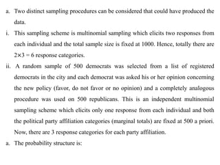
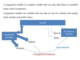
Thus, the Pearson chi-squared and likelihood-ratio statistics for independence,
respectively, are
𝑋2 = 𝑖=1
𝑟
𝑗=1
𝑐 (𝑛𝑖𝑗−µ𝑖𝑗)2
µ𝑖𝑗
~ 𝑋2 [(r-1) (c-1)] and
𝐺2
= 𝑖=1
𝑟
𝑗=1
𝑐
𝑛𝑖𝑗 log(
𝑛𝑖𝑗
µ𝑖𝑗
) ~ 𝑋2
[(r-1) (c-1)]
Example 2.3: The following cross classification shows the distribution of patients
by the survival outcome (active, dead, transferred to other hospital and loss-to-
follow) and gender. Test whether the survival outcome depends on gender or not
using both the Pearson and likelihood-ratio tests.
Gender Survival Outcome
Active Dead Transferred Loss-to-follow Total
Female 741 25 63 101 930
Male 392 20 52 70 534
Total 1133 45 115 171 1464

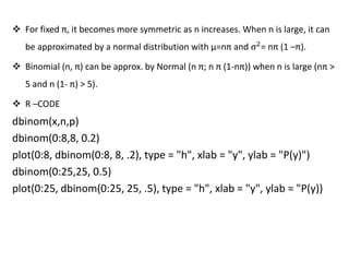
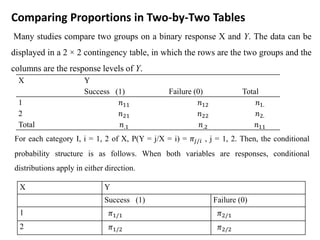
Solution: First let’s find the expected cell counts,
𝑛𝑖.𝑛.𝑗
𝑛
Gender Survival Outcome
Active Dead Transferred Loss-to-follow Total
Female 741 (719.7) 25 (28.6) 63 (73.1) 101 (108.6) 930
Male 392 (413.3) 20 (16.4) 52 (41.9) 70 (62.4) 534
Total 1133 45 115 171 1464
Thus, the Pearson chi-squared statistics is
𝑋2 = 𝑖=1
𝑟
𝑗=1
𝑐 (𝑛𝑖𝑗−µ𝑖𝑗)2
µ𝑖𝑗
=
(741−719.7)2
719.7
+
(25−28.6)2
28.6
+…+
(70−62.4)2
62.4
= = 8.2172
Since both statistics have larger values than 𝑋2 [(2-1) (4-1)] = 𝑋2
𝛼=0.05 (3), it can
be concluded that the survival outcome of patients depends on the gender.

Comparing Proportions in Two-by-Two Tables
Many studies compare two groups on a binary response X and Y. The data can be
displayed in a 2 × 2 contingency table, in which the rows are the two groups and the
columns are the response levels of Y.
X Y
Success (1) Failure (0) Total
1 𝑛11 𝑛12 𝑛1.
2 𝑛21 𝑛22 𝑛2.
Total 𝑛.1 𝑛.2 𝑛11
For each category I, i = 1, 2 of X, P(Y = j/X = i) = 𝜋𝑗/𝑖 , j = 1, 2. Then, the conditional
probability structure is as follows. When both variables are responses, conditional
distributions apply in either direction.
X Y
Success (1) Failure (0)
1 𝜋1/1 𝜋2/1
2 𝜋1/2 𝜋2/2

 Here, 𝜋1/1 and 𝜋1/2 are the proportions of successes in category 1 and 2 of X,
respectively.
 In chi-square test, the question of interest is whether there is a statistical
association between the explanatory X and the response variable Y.
 The hypothesis to be tested is
H0 : 𝜋1/1 = 𝜋1/2 ⟺ 𝜋2/1 = 𝜋2/2 (There is an no association between X and Y )
H1 : 𝜋1/1 ≠ 𝜋1/2 ⟺ 𝜋2/1 ≠ 𝜋2/2 (There is association between X and Y )

. Difference of Proportions
For subjects in row 1, let 𝜋1 denote the probability of a success, so 1 − 𝜋1 is the
probability of a failure.
For subjects in row 2, let 𝜋2 denote the probability of success.
The difference of proportions 𝜋1 − 𝜋2 compares the success probabilities in the two
groups. This difference falls between −1 and +1.
Let 𝜋1 and 𝜋2 denote the sample proportions of successes.
The sample difference 𝜋1 - 𝜋2 estimates 𝜋1 − 𝜋2.
When the counts in the two rows are independent binomial samples, the estimated
standard error of 𝜋1 - 𝜋2 is
SE (𝜋1 - 𝜋2) =
𝜋1 (1−𝜋1
𝑛1
+
𝜋2 (1−𝜋2)
𝑛2
The standard error decreases, and hence the estimate of 𝜋1 − 𝜋2 improves, as the
sample sizes increase.
A large-sample 100(1 − α) % (Wald) confidence interval for 𝜋1 − 𝜋2 is
(π1 - π2 ) ± zα/2SE (𝜋1 − 𝜋2)

Example 2.4: The following table is from a report on the relationship between aspirin use
and myocardial infarction (heart attacks) by the Physicians’ Health Study Research Group at
Harvard Group Myocardial Infarction
Yes No Total
Placebo 189 10,845 11,034
Aspirin 104 10,933 11,037
Of the n1 = 11,034 physicians taking placebo, 189 suffered myocardial infarction (MI) during
the study, a proportion of 𝜋1 = 189/11,034 = 0.0171. Of the n2 = 11,037 physicians taking
aspirin, 104 suffered MI, a proportion of 𝜋2 = 0.0094. The sample difference of proportions
is 0.0171 − 0.0094 = 0.0077 has an estimated standard error of
SE=
0.0171∗ 0.9829
11,034
+
0.0094 (0.9906 )
11,034
= 0.0015
A 95% confidence interval for the true difference π1 − π2 is 0.0077 ± 1.96(0.0015), which is
0.008 ± 0.003, or (0.005, 0.011). Since this interval contains only positive values, we
conclude that 𝜋1 − 𝜋2> 0, that is, 𝜋1 > 𝜋2. For males, taking aspirin appears to result in a
diminished risk of heart attack.

Relative Risk
Relative risk is a ratio of the probability of an event occurring in the
exposed group versus the probability of the event occurring in the non-
exposed group.
It is ratio of the probability that the outcome characteristic is present for one
group relative to the other group.
Relative Risk = (incidence in exposed group) / (incidence in not exposed group)
RR = RR =
𝜋1/1
𝜋1/2
=
𝑎/ 𝑎+𝑏
𝑐/(𝑐+𝑑)
=
𝑎(𝑐+𝑑)
𝑐(𝑎+𝑏)
=
𝑛11 𝑛2.
𝑛21 𝑛1.
similarly, the relative risk for
failures is RR =
1−𝜋2/1
1− 𝜋1/2
. The value of relative risk is non-negative.
If r ≈ 1, the proportion of successes in the two groups of X are the
same (corresponds to independence).

The sample relative risk (rr) =
𝜋1/1
𝜋1/1
estimates the population relative risk (RR).
If the probability of successes are equal in the two groups being compared, then r = 1
or log(r) = 0 indicating no association between the variables. Thus, under H0: log(r)
= 0, for large values of n the test statistic:
Z=
log 𝑟 −log(𝑅𝑅)
𝑺𝑬[𝐥𝐨𝐠(𝐫)]
~N (0, 1)
Thus, the 100 (1-α) % confidence interval for log(r) is given by
[log (r)] ± 𝑧𝛼/2𝑆𝐸[log(r)].
Were, 𝑆𝐸[log(rr)]=
1
𝑛11
+
1
𝑛11
+
1
𝑛1.
+
1
𝑛2.
Taking the exponentials of the end points this confidence interval provides the
confidence interval for RR: exp{log (r) ± 𝑧𝛼/2𝑆𝐸[log(r)}.

Example 2.5: Consider the following table categorizing students by their academic
performance on a statistics course examination (pass or fail) to two different
teaching methods (teaching using slides or lecturing on the board). Find
a. The relative risk for the data and test its significance.
b. The 100 (1-α) % confidence interval
Teaching Methods Examination Result
Pass Fail Total
Slide 45 20 65
Lecturing 32 3 35
Total 77 23 100
The estimate of the relative risk is (rr) =
𝜋1/1
𝜋1/1
=
45∗35
32∗65
=
0.692
0.914
= 0.757,
Which implies log(r) = log(0.757) = -0.2784 and
𝑆𝐸[log(r)]=
1
45
+
1
32
+
1
65
+
1
35
= 0.0095 = 0.0975

Thus, the 100 (1-α) % confidence interval for log(r) is given by
[log (r)] ± 𝑧𝛼/2𝑆𝐸[log(r)].
(-0.2784 ± 1.96*0.0975) = (-0.2784 ± 0.1911)
= (-0.4695, -0.0873)
The value of confidence interval doesn’t include 1. Therefore, the relative risk is
significantly different from 1.
Thus, it can be concluded that the proportion of passing in the slide group is 0.757
times that of the lecturing group.
Or by inverting, the probability of passing in the lecturing group is 𝑒0.32
= 1.377
times that of the slide teaching method group.

Odds Ratio
An odds is the ratio of the probability of success to the probability of failure in a
particular group. The odds of an event is the number of events / the number of
non-events.
Odds =
𝑝(𝑠𝑢𝑐𝑐𝑒𝑠𝑠)
𝑝(𝑓𝑎𝑖𝑙𝑢𝑟𝑒)
=
𝜋
1−𝜋
=
𝑛𝑢𝑚𝑏𝑒𝑟 𝑜𝑓 𝑠𝑢𝑐𝑐𝑒𝑠𝑠
𝑛𝑢𝑚𝑏𝑒𝑟 𝑜𝑓 𝑓𝑎𝑖𝑙𝑢𝑟𝑒
An odds is a nonnegative number ≥ 0.
If odds ≈ 1, a probability of successes is equally likely as a probability of failure.
If 0 < odds <1, a probability of success is less likely as a probability of failure
and;
If 1 < odds < ∞, a probability of success is more likely to occur than a probability
of failure.

An odds ratio (OR) is a measure of association between an exposure and an
outcome.
OR =
𝑜𝑑𝑑𝑠1
𝑜𝑑𝑑𝑠2
=
𝜋1
/(1 − 𝜋1
)
𝜋2/(1 − 𝜋2)
=
𝜋11/𝜋12
𝜋21/𝜋22
=
𝜋11𝜋22
𝜋12𝜋21
=
𝑎𝑑
𝑏𝑐
, is the odds ratio.
Whereas, the relative risk is a ratio of two probabilities, the odds ratio (OR) is a
ratio of two odds.
 The odds ratio can also be used to determine whether a particular
exposure is a risk factor for a particular outcome, and to compare
the magnitude of various risk factors for that outcome.
OR=1 Exposure does not affect odds of outcome
OR>1 Exposure associated with higher odds of outcome
OR<1 Exposure associated with lower odds of outcome

Inference for Odds Ratios and Log Odds Ratios
Unless the sample size is extremely large, the sampling distribution of the odds
ratio is highly skewed.
The log odds ratio is symmetric about zero, in the sense that reversing rows or
reversing columns changes its sign.
The sample log odds ratio, log 𝜃, has a less skewed sampling distribution that is
bell-shaped. Its approximating normal distribution has a mean of log θ and a
standard error of 𝑆𝐸 =
1
𝑛11
+
1
𝑛11
+
1
𝑛12
+
1
𝑛22
,
The SE decreases as the cell counts increase
A large-sample confidence interval for log θ is log 𝜃 ± 𝑧𝛼/2𝑆𝐸 (log 𝜃),
Exponentiation endpoints of this confidence interval yields one for θ.

Example 2.6: The following table is from a report on the relationship between
aspirin use and myocardial infarction (heart attacks) by the Physicians’ Health
Study Research Group at Harvard
Group Myocardial Infarction
Yes No Total
Placebo 189 10,845 11,034
Aspirin 104 10,933 11,037
a. Find estimated odds of MI
b. Odds ratio
c. Find 95% CI for OR
a. The estimated odds of MI equal n11/n12 = 189/10,845 = 0.0174.
Since 0.0174 = 1.74/100, the value 0.0174 means there were 1.74 “yes”
outcomes for every 100 “no” outcomes.
The estimated odds for those taking aspirin equals 104/10,933 = 0.0095, Since,
0.95 “yes” outcomes per every 100 no” outcomes.

b. The sample odds ratio equals 𝜃 = 0.0174/0.0095 = 1.832. This also equals the
cross-product ratio
𝑛11𝑛22
𝑛12𝑛21
=
189 × 10,933
10,845 × 104
= 1.832.
The estimated odds of MI for male physicians taking placebo equal 1.83 times
the estimated odds for male physicians taking aspirin.
The estimated odds were 83% higher for the placebo group.
c,. The natural log of 𝜃 equals log(1.832) = 0.605. From (2.5), the SE of log 𝜃
equals 𝑆𝐸 =
1
189
+
1
10933
+
1
104
+
1
10845
= 0.123

 For the population, a 95% confidence interval for log θ equals
0.605 ± 1.96(0.123), or (0.365, 0.846).
 The corresponding confidence interval for θ is [exp(0.365),
exp(0.846)] = (e0.365, e0.846) = (1.44, 2.33).
Since the confidence interval (1.44, 2.33) for θ does not contain
1.0, the true odds of MI seem different for the two groups.
 We estimate that the odds of MI are at least 44% higher for
subjects taking placebo than for subjects taking aspirin.

Relationship between Odds Ratio and Relative Risk
Odds ratio =
𝜋1/(1 − 𝜋1)
𝜋2/(1 − 𝜋2)
= Relative risk *
1− 𝜋1
1− 𝜋1
This relationship between the odds ratio and the relative risk is useful. For some
data sets direct estimation of the relative risk is not possible, yet one can estimate
the odds ratio and use it to approximate the relative risk.

Chi-square tests of independence
The test statistics used to make such comparisons have large-sample chi-squared
distributions.
The Pearson chi-squared statistic for testing H0 is
X2 =
nij − µij
2
µij
The chi-squared distribution is concentrated over nonnegative values.
It has mean equal to its degrees of freedom (df), and its standard deviation equals
(2df )

Reading assignment
1. Chi-square test of homogeneity
2. Chi-square test of goodness-of-fit
3. Likelihood-Ratio Statistic
4. Association in three-way tables
5. Testing for independence for ordinal data

CHAPTER THREE
LOGISTIC REGRESSION
 Regression methods have become an integral component of any data analysis
concerned with describing the relationship between a response variable and
one or more explanatory variables.
 It is often the case that the outcome variable is continuous, taking on two or
more possible values.
 Logistic regression describes the relationship between a dichotomous response
variable and a set of explanatory variables.
 Here, the response variable Y takes the value 1 for success with probability π
and it takes the value 0 for failure with probability 1 -π.

Logistic regression
Logistic regression is a mathematical modeling approach that can be used to
describe the relationship of several X’s to a dichotomous dependent variable.
 It is the most popular modeling procedure used to analyze epidemiologic data
when the response variable is dichotomous.
 The fact that the logistic function f(z) ranges between 0 and 1 is the primary
reason the logistic model is so popular.
 The model is designed to describe a probability, which is always some number
between 0 and 1.
 In epidemiologic terms, such a probability gives the risk of an individual
getting a disease.

Thus, as the graph describes, the range of f(z) is between 0 and 1, regardless of the
value of z.
Range: 0 ≤ f(z) ≤ 1 and 0 ≤ probability (individual risk) ≤ 1
Another reason why the logistic model is popular derives from the shape of the
logistic function.

So, the logistic model is popular because the logistic function, on which the
model is based, provides:
 Estimates that must lie in the range between zero and one
 An appealing S-shaped description of the combined effect of several risk
factors on the risk for a disease.

The logistic regression model
For a binary response 𝑌𝑖 and a quantitative explanatory variable 𝑥𝑖, i=1, 2, . . . , k,
let πi = P(𝑥𝑖) denote the “success probability” when 𝑋𝑖 take the values xij.
Where, π𝑖 = P (𝑌𝑖 =1) within the interval 0 and 1
f (z)=
𝟏
𝟏+𝐞−𝐳 = f (z) =
𝟏
𝟏+𝐞−(𝛂+𝛃𝟏𝐱𝟏+𝛃𝟐𝐱𝟐+⋯.+𝛃𝐤𝐱𝐤)= f (z)=
𝟏
𝟏+𝐞−(𝛂+ 𝛃𝐱𝐢)............. 3.1
Note that 0 ≤ f(z) ≤1.
Hence, to indicate that it is a probability value, the notation π(𝒙𝒊) can be used instead.
That is, π(𝐗𝐢) =
𝟏
𝟏+𝐞−(𝛂+𝛃𝐱𝐢) , π(xi) = P(Y=1/𝐗𝐢=𝐱𝐢) = 1- P(Y=0/𝐗𝐢=𝐱𝐢)............. 3.2
It can also be written as π(𝒙𝒊) =
𝑒(α+βxi)
1+𝑒(α+βxi)
The probability being modeled can be denoted by the conditional probability
statement P(Y=1/x1, x2, . . . , xk).

Therefore, we apply the logit transformation where the transformed quantity lies in
the interval from minus infinity to positive infinity and it is modeled as
The logit (πi) = log (
𝛑𝐢
𝟏−𝛑𝐢
) = 𝐳 = 𝛂 + 𝛃𝟏𝐱𝟏 + 𝛃𝟐𝐱𝟐 + ⋯ . +𝛃𝐤𝐱𝐤.................. 3.3
The Logit Transformation
The logit of the probability of success is given by the natural logarithm of the odds
of successes.
Therefore, the logit of the probability of success is a linear function of the
explanatory variable.
Thus, the simple logistic model is logit (π(𝑋𝑖)) = Log [
π(𝑋𝑖)
1−π(𝑋𝑖)
] = α + βxi
The probit model or the complementary log-log model might be appropriate when
the logit model does not fit the data well.

The link function
Function form Typical application
Logit Log [
π(𝑋𝑖)
1−π(𝑋𝑖)
] Evenly distributed categories
Complementary log-log Log [-Log (1-
π(𝑋𝑖))]
Higher categories are more
probable
Negative log-log -Log π(𝑋𝑖) Lower categories are more
probable
Probit 𝜙−1
[π(𝑋𝑖)] Normally distributed latent
variable

Interpretation of the Parameters
The logit model is monotone depending on the sign of β.
Its sign determines whether the probability of success is increasing or decreasing as
the value of the explanatory variable increases.
Thus, the sign of β indicates whether the curve is increasing or decreasing. When β
is zero, Y is independent of X.
Then, π(xi) =
exp(α)
1+exp(α)
, is identical for all xi, so the curve becomes a straight line.
The parameters of the logit model can be interpreted in terms of odds ratios.
From logit [π(xi)] = α + βxi, an odds is an exponential function of xi. This provides a
basic interpretation for the magnitude of β.

 If odds = 1, then a success is as likely as a failure at the particular value 𝒙𝒊 of the
explanatory variable.
 If odds > 1) log [odds] > 0, a success is more likely to occur than a failure.
 On the other hand, if odds < 1, log [odds] < 0, a success is less likely than a
failure.
Thus, the odds ratio is
𝑜𝑑𝑑𝑠(xi+1)
𝑜𝑑𝑑𝑠(xi)
= exp(β) This value is the multiplicative effect of
the odds of successes due to a unit change in the explanatory variable.
The intercept α is, not usually of particular interest, used to obtain the odds at xi= 0.

Example 3.1: The study conducted on the factor of TB patients (coded as 1 for
alive and 0 for died) using the explanatory variable age, taking a sample of 154
individuals were examined at Debre Tabor referral hospital. Find
a. Write the model that allows the prediction of the probability of having TB
patients at a given age. Also write out the estimated logit model.
b. What is the probability of having TB at the age of 35? Also find the odds of
having TB at this age.
c. What is the estimated odds ratio of having TB and interpret.
d. Find the median effective level (EL50) and interpret.
e. If the mean age is 36.3, find the probability of success at the sample mean and
determine the incremental change at this point.

The analysis also done using R statistical software, the following parameter estimates were
obtained.
Coefficients:
Estimate Std. Error z value exp(β) Pr(>|z|)
(Intercept) -3.44413 0.64171 -5.367 0.03193 8.0e-08 ***
Age 0.05692 0.01253 4.541 1.0568 5.6e-06 ***
Signif. codes: 0 ‘***’ 0.001 ‘**’ 0.01 ‘*’ 0.05 ‘.’ 0.1
Let Y = TB and X= age. Then 𝜋(xi)= 𝑝 (Y = 1/xi) is the estimated probability of
having TB, Y = 1, given the age xi of an individual i.
a. π(xi) =
𝑒(−3.44413 +0.05692 age)
1+𝑒(−3.44413 +0.05692) Also, the estimated logit model is written as
Logit [𝜋(xi)]= log[
𝜋(xi)
1−𝜋(xi)
] = −3.44413 + 0.05692 age
b. The probability of having pneumonia at the age of 35 years is
𝜋 (35)=
𝑒(−3.44413 +0.05692(35))
1+𝑒(−3.44413 +0.05692(35)) =
0.0338
1.0338
= 0.0327 and its odds =
𝑒(−2.844+0.05692 age)= 0.0338

c. The odds (risk) of having TB is exp(𝛽) = exp(0.05692) = 1.0568 times larger
for every year older an individual. In other words, as the age of an individual
increases by one year, the odds (risk) of developing TB increases by a factor of
1.0568. Or it can be said the odds (risk) of having pneumonia increases by [exp
(0.05692) - 1] × 100% = 5.6%.
d. The median effective level, the age at which an individual has a 50% chance of
having pneumonia, is EL50 =
−𝛼
𝛽
=
−(−3.44413)
0.05692
= 60.508 years.
e. The probability of having TB at the mean age of 35 years that the mean given
as βπ(xi)[1- π(xi)] = 0.0327(1-0.0327) 0.05692 = 0.0018

Logit Models with Categorical Predictors
If there is a categorical explanatory variable with two or more categories, then it is
inappropriate to include it in the model as if it was quantitative.
• In such case, a set of categorical variables, called design (dummy indicator),
should be created to represent quantitative variables.
• For example, the explanatory variable “marital status” with three categories;
"Single", "Married", "divorced" and “windowed”.
Design variables
Marital status d1 d2 d3 d4
Single 0 0 0 0 Reference
Married 1 0 0 0 Married when the other is 0
Divorced 0 1 0 0 divorced when the other is 0
Windowed 0 0 1 0 windowed when the other is 0

Thus, the logit model would be:
Logit(π(𝐱𝐢)) = α + 𝛃𝟏𝐝𝐢𝟏 + 𝛃𝟐𝐝𝐢𝟐 + , . . ., +𝛃𝐦−𝟏𝐝𝐢,𝐦−𝟏............. 3.4
Example 3.2: For studying the effect of residence (0 = male, 1= female) on the
occurrence of TB (coded as 1 for alive and 0 for died), a sample of 154 individuals
were examined at Debre Tabor referral hospital. The analysis also done using R
statistical software, the following parameter estimates were obtained.
(Intercept) -1.1508 0.2306 -4.990 0.3164 6.05e-07 ***
Residence 0.9485 0.3318 2.859 2.582 0.00425 **
Signif. codes: 0 ‘***’ 0.001 ‘**’ 0.01 ‘*’ 0.05 ‘.’ 0.1 ‘ ’ 1

 The log probability of patients died by TB disease among residence of urban
is -1.1508 and residence of rural is 0.9485.
 The odds ratio for a residence of rural is 0.9485 and thus the odds rural of
2.582 times more likely to have TB disease death as compared to urban
residence.
 Or residence of rural is exp (𝛽) = exp (0.9485) = 2.582 times more likely to
have TB disease death as compared to urban residence.

Multiple Logistic Regressions
Suppose there are k explanatory variables (categorical, continuous or both) to be
considered simultaneously.
𝐳𝐢= 𝛃𝟎 + 𝛃𝟏𝐱𝐢𝟏 + 𝛃𝟐𝐱𝐢𝟐 + …+ 𝛃𝐩𝐱𝐢𝐤.
Consequently, the logistic probability of success for subject i given the values of the
explanatory variables
𝐱𝐢 = (𝐱𝐢𝟏, 𝐱𝐢𝟐, …, 𝐱𝐢𝐤) is π (𝐱𝐢) =
𝟏
𝟏+𝐞𝐱𝐩[−(𝛃𝟎 + 𝛃𝟏𝐱𝐢𝟏 + 𝛃𝟐𝐱𝐢𝟐 + …+ 𝛃𝐩𝐱𝐢𝐤 )]
, where
π (𝒙𝒊) =p (𝒀𝒊=1/𝒙𝒊𝟏, 𝒙𝒊𝟐, …, 𝒙𝒊𝒌)= logit [π (𝒙𝒊)] = log (
𝛑 (𝒙𝒊)
𝟏− 𝛑 (𝒙𝒊)
) = 𝜷𝟎 + 𝜷𝟏𝒙𝒊𝟏 +
𝜷𝟐𝒙𝒊𝟐 + …+ 𝜷𝒑𝒙𝒊𝒌
Similar to the simple logistic regression, exp(𝛽𝑖) represents the odds ratio associated
with an exposure if 𝑥𝑗 is binary (exposed 𝑥𝑖𝑗 = 1 versus unexposed 𝑥𝑖𝑗 = 0); or it is the
odds ratio due to a unit increase if 𝑥𝑗 is continuous (𝑥𝑖𝑗 = 𝑥𝑖𝑗 + 1 versus 𝑥𝑖𝑗 = 𝑥𝑖𝑗).

Example 3.3: For studying the effect of residence (0 = male, 1= female) and age on
the occurrence of TB (coded as 1 for alive and 0 for died), a sample of 154
individuals were examined at Debre Tabor referral hospital. The analysis also done
using R statistical software, the following parameter estimates were obtained.
Coefficients:
(Intercept) -3.50307 0.65420 -5.355 0.0301 8.57e-08 ***
Residence (Urban) 0.59879 0.39749 1.506 1.8200 0.0132
Age 0.05252 0.01261 4.165 1.0539 3.11e-05 ***
Signif. codes: 0 ‘***’ 0.001 ‘**’ 0.01 ‘*’ 0.05 ‘.’ 0.1 ‘ ’ 1
Residence of rural is exp (𝛽) = exp (0.9485) = 1.820 times more likely to have TB
disease death as compared to urban residence when the other factor become constant.
As the age of an individual increases by one year the odds (risk) of developing TB
death increases by a factor of 1.0539 when the other factor held constant.

Inference for Logistic Regression
Parameter Estimation
The goal of logistic regression model is to estimate the k + 1 unknown parameters
of the model. This is done with maximum likelihood estimation which entails
finding the set of parameters for which the probability of the observed data is
largest.
 Then each binary response Yi, i = 1, 2, …, m has an independent Binomial
distribution with parameter ni and π(xi), that is,
P (𝐘𝐢 =𝐘𝐢) =
𝐧𝐢!
(𝐧𝐢−𝐲𝐢)! 𝐲𝐢!
[𝛑(𝐱𝐢)]𝐲𝐢 [𝟏 − 𝛑(𝐱𝐢)]𝐧𝐢−𝐲𝐢, 𝐲𝐢 = 1,2,…, 𝐧𝐢 …..3.6
Where, 𝑥𝑖 = (𝑥𝑖1, 𝑥𝑖2, …, 𝑥𝑖𝑘) for population i
Then, the joint probability mass function of the vector of m Binomial random
variables, 𝑌𝑖 = (𝑌1, 𝑌2, …, 𝑌𝑚), is the product of the m Binomial distributions:

P (y/β) = 𝑖=1
𝑚 𝑛𝑖!
(𝑛𝑖−𝑦𝑖)! 𝑦𝑖!
[π(xi)]𝑦𝑖 [1 − π(xi)]𝑛𝑖−𝑦𝑖 ……..3.7
The likelihood function has the same form as the probability mass function, except
that it expresses the values of β in terms of known, fixed values for y. Thus,
ʟ (β/y) = 𝑖=1
𝑚 𝑛𝑖!
(𝑛𝑖−𝑦𝑖)! 𝑦𝑖!
[π(xi)]𝑦𝑖 [1 − π(xi)]𝑛𝑖−𝑦𝑖 …….3.8
maximizing the equation without the factorial terms will come to the same result as
if they were included. Therefore, equation (3.7) can be written as:
ʟ (β/y) = 𝑖=1
𝑚
[π(xi)]𝑦𝑖 [1 − π(xi)]𝑛𝑖−𝑦𝑖 , and it can be re-arranged as:
ʟ (β/y) = 𝒊=𝟏
𝒎
[
𝛑(𝐱𝐢)
𝟏−𝛑(𝐱𝐢)
]𝒚𝒊 [𝟏 − 𝛑(𝐱𝐢)]𝒏𝒊 …………….............. 3.8
By substituting the odds of successes and probability of failure in equation (3.8),
the likelihood function becomes
ʟ (β/y) = 𝒊=𝟏
𝒎
[𝐞𝐱𝐩(𝒚𝒊 𝒋=𝟏
𝒌
𝛃𝒋 𝒙𝒊𝒋)] [𝟏 + 𝐞𝐱𝐩( 𝒋=𝟏
𝒌
𝛃𝒋 𝒙𝒊𝒋)]−𝒏𝒊 ............ 3.9

Thus, taking the natural logarithm of equation (3.9) gives the log-likelihood
function:
ʟ (β/y) = 𝐢=𝟏
𝐦
𝒚𝒊 𝒋=𝟏
𝒌
𝜷𝒋 𝒙𝒊𝒋 −𝒏𝒊 𝐥𝐨𝐠[𝟏 + 𝐞𝐱𝐩 𝒋=𝟏
𝒌
𝛃𝒋 𝒙𝒊𝒋 ]..... 3.10
To find the critical points of the log-likelihood function, first, equation (3.9) should
be partially differentiated with respect to each 𝛽𝑗, j = 0, 1, … k
Əʟ (β/y)
Ə𝜷𝒋
= 𝒊=𝟏
𝒎
[𝒚𝒋 𝒙𝒊𝒋 - 𝒏𝒊𝝅𝒊(𝒙𝒊) 𝒙𝒊𝒋]= 𝒊=𝟏
𝒎
[𝒚𝒋- 𝒏𝒊𝝅𝒊(𝒙𝒊) ]𝒙𝒊𝒋 , j= 0, 1, 2, …, k…...3.11
Since the second partial derivatives of the log-likelihood function:
Ə2ʟ (β/y)
Ə𝜷𝒋Ə𝜷𝒉
= - 𝒊=𝟏
𝒎
𝒏𝒊𝝅𝒊(𝒙𝒊) [1- 𝝅𝒊(𝒙𝒊)] 𝒙𝒊𝒋𝒙𝒊𝒉 , j,h= 0,1,2,…, k…………….3.22

Goodness-of-Fit Tests
Overall performance of the fitted model can be measured by several different goodness-of-fit tests.
Two tests that require replicated data (multiple observations with the same values for all the predictors) are
the Pearson chi-square goodness-of-fit test and the deviance goodness-of-fit test (analogous to the
multiple linear regression lack-of-fit F-test).
Both of these tests have statistics that are approximately chi-square distributed with c - k - 1 degrees of
freedom, where c is the number of distinct combinations of the predictor variables.
When a test is rejected, there is a statistically significant lack of fit. Otherwise, there is no evidence of lack
of fit.
By contrast, the Hosmer-Lemeshow goodness-of-fit test is useful for un-replicated datasets or for
datasets that contain just a few replicated observations.
For this test the observations are grouped based on their estimated probabilities.
The resulting test statistic is approximately chi-square distributed with c - 2 degrees of freedom, where c is
the number of groups (generally chosen to be between 5 and 10, depending on the sample size).

The final measure of model fit is the Hosmer and Lemeshow goodness-of-fit
statistic, which measures the correspondence between the actual and predicted
values of the dependent variable (Hosmer, D., 2000).
Pearson Chi-square statistics(X2)
X2=
Oij−Nij 2
Nij
where Oij is each observation values of the cell
Hosmer and Lemeshow Test
Step Chi-square df Sig.
1 5.320 8 .723
From the above table 4.6 above Hosmer and Lemeshow test p value (0.723) are greater than 0.05 since
we do not reject HO. Therefore the model is good fit.
In other words the Hosmer-Lemeshow goodness-of-fit statistic is not association indicating that we do
not have an evidence to reject the null hypothesis, suggesting that the model fitted the data well.

Likelihood-Ratio Test of Model Fit
Suppose two alternative models are under consideration, one model is simpler or
more parsimonious than the other.
A common situation is to consider ‘nested’ models, where one model is obtained
from the other one by putting some of the parameters to be zero. Suppose now we
test
Ho: reduced model is true vs. H1: current model is true
Let 𝐿𝑜denote the maximized value of the likelihood function of the null model
which has only one parameter, that is, the intercept.
Also let 𝐿𝑚 denote the maximized value of the likelihood function of the model M
with all explanatory variables (having k + 1 parameters). Then, the likelihood-
ratio test statistic is 𝐺2 = -2Log (
𝐿𝑜
𝐿𝑚
) = -2 (Log𝐿𝑜- Log𝐿𝑚) ~𝑋2(k)

• The Cox & Snell R2 indicates that 44.1% of the dependent variables is
explained by the independent variables. In addition to this, Nagelkerke’s R2
indicates that 59.0 % of the dependent variable is also explained by the
independent variable.
Model Summary
Step -2 Log likelihood Cox & Snell R Square Nagelkerke R Square
1 191.257a .441 .590

Wald Test for Parameters
The Wald test is used to identify the statistical significance of each
coefficient (𝛽𝑗) of the logit model. That is, it is used to test the null
hypothesis
H0 : 𝛽𝑗 = 0 which states that factor 𝛽𝑗 does not have significant value
added to the prediction of the response given that other factors are already
included in the model.
The Wald statistic calculates a Z statistic in which
𝑧𝑗 =
𝛽𝑗
𝑠𝑒(𝛽𝑗)
~ N (0, 1), for large sample size.
𝑧𝑗
2 = (
𝛽𝑗
𝑠𝑒(𝛽𝑗)
)2 ~ 𝑋2(1)

Confidence Intervals
Confidence intervals are more informative than tests. A confidence interval for 𝛽𝑗
results from inverting a test of H0: 𝛽𝑗 = 𝛽𝑗0.
The interval is the set of 𝛽𝑗0's for which the z test statistic is not greater than 𝛽Ə/2.
For the Wald approach, this means
𝛽𝑗−𝛽𝑗0
𝑆𝐸(𝛽𝑗)
≤ 𝑧Ə/2
This yields the confidence interval 𝛽𝑗 ± 𝑧Ə/2SE(𝛽𝑗) 𝛽𝑗, j= 1, 2, . . ., k. As the
point estimate of the odds ratio associated to 𝑋𝑗 is exp (𝛽𝑗) and its confidence
interval is exp[𝛽𝑗 ± 𝑧Ə/2SE(𝛽𝑗)].

Chapter 4
Building and Applying Logistic Regression Models
Model Selection
With several explanatory variables, there are many potential models.
The model selection process becomes harder as the number of explanatory variables
increases, because of the rapid increase in possible effects and interactions.
There are two competing goals of model selection.
The model should be complex enough to fit the data well.

Likelihood-Ratio Model Comparison Test
Let 𝐿𝑚 denote the maximized value of the likelihood function for the model of
interest M with pM =k+1 parameters and let 𝐿𝑅 denote the maximized value of the
likelihood function for the reduced model R with pR = k + 1 - q parameters.
Note that model R is nested under model M. Thus, the null hypothesis
Ho: 𝛽0 = 𝛽1 =𝛽2 = …= 𝛽𝑘 = 0, there is no contribution of all the q predictors in
model M is tested using
𝐺2= -2[(log(𝐿𝑅) - log(𝐿𝑚) ~𝐺2(q)
where, 𝐿𝑚= L(𝛽0, 𝛽1, 𝛽2, ... , 𝛽𝐾) and 𝐿𝑅= L(𝛽0, 𝛽𝑞+1, 𝛽𝑞+2,.. ., 𝛽𝑘)

Akaike and Bayesian Information Criteria
Deviance or likelihood-ratio tests are used for comparing nested models.
When there are non nested models, information criteria can help to select the good
model.
The best known ones are the Akaike Information Criterion (AIC) and Bayesian
Information Criteria (BIC).
Both judge a model by how close its fitted values tend to be to the true expected
values.
Also, both are calculated based on the likelihood value of a particular model M as
AIC = -2 log𝐿𝑚+ 2P
BIC = -2 log𝐿𝑚+ p log(n), where P is number of parameters in the model and n is
the sample size.
A model having smaller AIC or BIC is better.

Measures of Predictive Power
Let the maximized likelihood be denoted by 𝐿𝑚 for a given model, 𝐿𝑠 for the
saturated model and 𝐿0 for the null model containing only an intercept term.
These probabilities are not greater than 1, thus log-likelihoods are non-positive.
As the model complexity increases, the parameter space expands, so the
maximized log-likelihood increases. Thus,
𝐿0 ≤ 𝐿𝑚 ≤ 𝐿𝑠 ≤ 1 or Log𝐿0 ≤ 𝐿𝑜𝑔𝐿𝑚 ≤ Log𝐿𝑠 ≤ 0 or
𝑅2 =
𝐿𝑜𝑔𝐿𝑚−Log𝐿0
𝐿𝑜𝑔𝐿𝑠−Log𝐿0
,
The measure lies between 0 and 1. It is zero when the model provides no
improvement in fit over the null model and it will be 1 when the model fits as
well as the saturated model.

The McFadden 𝑹𝟐
Since the saturated model has a parameter for each subject, the log𝐿𝑠 approaches to
zero. Thus, log𝐿𝑠 = 0 simplifies
𝑅2
McFadden=
𝐿𝑜𝑔𝐿𝑚−Log𝐿0
−Log𝐿0
= 1- [
𝐿𝑜𝑔𝐿𝑚
Log𝐿0
]
The Cox & Snell 𝑹𝟐
The Cox & Snell modified 𝑅2 is:
𝑅2
Cox−Snell = 1-
𝐿0
𝐿𝑚
2/𝑛
= 1- exp(Log𝐿0 − 𝐿𝑜𝑔𝐿𝑚) 2/𝑛
The Nagelkerke 𝑹𝟐
Because the 𝑅2
Cox−Snell value cannot reach 1, Nagelkerke modified
it. The correction increases the Cox & Snell version to make 1 a
possible value for 𝑅2
.
𝑅2
Nagelkerke =
1−
𝐿0
𝐿𝑚
2/𝑛
1−(𝐿0)2/𝑛 =
1−(exp(Log𝐿0−𝐿𝑜𝑔𝐿𝑚))2/𝑛
1−[exp(𝐿0)]2/𝑛

Model Checking
For any particular logistic regression model, there is no guarantee that the model
fits the data well.
One way to detect lack of fit uses a likelihood-ratio test.
A more complex model might contain a nonlinear effect, such as a quadratic term
to allow the effect of a predictor to change directions as its value increases.
Models with multiple predictors would consider interaction terms.
If more complex models do not fit better, this provides some assurance that a
chosen model is adequate.

• Pearson Chi-squared Statistic
Suppose the observed responses are grouped into m covariate patterns
(populations). Then, the raw residual is the difference between the observed
number of successes 𝑦𝑖 and expected number of successes 𝑛𝑖π (𝑥𝑖) for each value
of the covariate 𝑥𝑖. The Pearson residual is the standardized difference. That is,
𝑟𝑖 =
𝑦𝑖−𝑛𝑖 𝜋 (𝑥𝑖)
𝑛𝑖 𝜋 𝑥𝑖 [1−𝜋 (𝑥𝑖)]
~ 𝑥2
(m-k)
• When this statistic is close to zero, it indicates a good model fit to the data.
When it is large, it is an indication of lack of fit. Often the Pearson residuals 𝑟𝑖
are used to determine exactly where the lack of fit occurs.

The Deviance Function
The deviance, like the Pearson chi-squared, is used to test the adequacy of the
logistic model. As shown before, the maximum likelihood estimates of the
parameters of the logistic regression are estimated iteratively by maximizing the
Binomial likelihood function.
The deviance is given by:
D = 2 𝑖=1
𝑚
𝑦𝑖 log
𝑦𝑖
𝑛𝑖π 𝑥𝑖
+ (𝑛𝑖 − 𝑦𝑖)𝑙𝑜𝑔
𝑛𝑖−𝑦𝑖
𝑛𝑖−𝑛𝑖π 𝑥𝑖
~ 𝑥2(m-k)
Where the fitted probabilities π 𝑥𝑖 satisfy logit [π 𝑥𝑖 ] = 𝑖
𝑘
𝛽𝑗 𝑥𝑖𝑗 and 𝑥𝑖0=1.
The deviance is small when the model fits the data, that is, when the observed
and fitted proportions are close together. Large values of D (small p-values)
indicate that the observed and fitted proportions are far apart, which suggests
that the model is not good.

• The chi-square of 5.272762 with 1 degrees of freedom and an associated p-
value of less than 0.02166161 tells us that our model as a whole fits
significantly better than an empty model. This is sometimes called a likelihood
ratio test (the deviance residual is -2*log likelihood). To see the model’s log
likelihood, we type:

Chapter Five
Multicategory Logit Models
In this chapter, the standard logistic model is extended to handle outcome
variables that have more than two categories.
Multinomial logistic regression is used when the categories of the outcome
variable are nominal, that is, they do not have any natural order.
When the categories of the outcome variable do have a natural order, ordinal
logistic regression may also be appropriate.

Multinomial Logit Model
 Let Y be a categorical response with J categories. Multinomial logit models for
nominal response variables simultaneously describe log odds for all
𝐽
2
pairs of
categories.
 Of these, a certain choice of J -1 are enough to determine all, the rest are
redundant.
 Let P(Y = j/xi) = 𝜋𝑗 (𝑥𝑖) at a fixed setting 𝑥𝑖 for explanatory variables with
𝑗=1
𝐽
𝜋(𝑥𝑖) =1
 Thus, Y has a multinomial distribution with probabilities 𝜋1(𝑥1), 𝜋2(𝑥2), . . .
𝜋𝐽(𝑥𝐽).

Baseline Category Logit Models
Log
𝜋𝑗 (𝑥𝑖)
𝜋𝐽 (𝑥𝑖)
= 𝛽𝑗0 + 𝛽𝑗1 𝑥𝑖1 + 𝛽𝑗2 𝑥𝑖2 + . . . + 𝛽𝑗𝑘 𝑥𝑖𝑘 , j = 1, 2, . . . , J-1
Simultaneously describes the effects of the explanatory variables on these J-1 logit
models.
The intercepts and effects vary according to the response paired with the baseline.
That is, each model has its own intercept and slope.
The J - 1 equations determine parameters for logit models with other pairs of
response categories, since
Log
𝜋1 (𝑥𝑖)
𝜋2 (𝑥𝑖)
= Log
𝜋1 𝑥𝑖 /𝜋𝐽 𝑥𝑖
𝜋2 (𝑥𝑖)/𝜋𝐽 𝑥𝑖
= log
𝜋1 (𝑥𝑖)
𝜋𝐽 (𝑥𝑖)
- log
𝜋2 (𝑥𝑖)
𝜋𝐽 (𝑥𝑖)

Example 5.1: Based the survival outcome of heart failure patient admitted at Debre
Tabor hospital (active, loss to follow up, dead). To identify factors associated with
these survival outcomes, a multinomial logit model was fitted. Two explanatory
variables that were considered are Age and residence (0= urban, 1= rural). The
parameter estimates are presented as follows.
let
π1 = probability of active,
π2 = probability of loss to follow up,
π3 = probability of died, and make “dead “be the baseline category.
The logit equations are:
Log
𝜋𝑗
𝜋3
= 𝛽𝑗0 + 𝛽𝑗1 𝑥𝑖1 + 𝛽𝑗2 𝑥𝑖2 + 𝛽𝑗3 𝑥𝑖3 , j = 1, 2

Multinomial logistic regression Number of obs = 154
LR chi2(6) = 46.60
Prob > chi2 = 0.0000
Log likelihood = -136.96831 Pseudo R2 = 0.1454
Logit Parameter Estimate Std. Err. z P>|z| [95% Conf.
Log (active vs. dead) or
log(𝜋𝑎𝑐𝑡𝑖𝑣𝑒 /𝑑𝑒𝑎𝑑 )
Intercept 4.296 .858 5.01 0.000 2.612 5.977
age -.0503 .0155 -3.24 0.001 -.082 -.0198
Residence (ref= urban) 1.409 .508 -2.77 0.006 -2.405 -.413
sex (ref = male) -.6042 .5490 -1.10 0.271 -1.680 .4718
Log (loss to follow up
vs. dead) or
log(𝜋𝑙𝑜𝑠𝑠− 𝑓𝑜𝑙𝑙𝑜𝑤 /𝑑𝑒𝑎𝑑 )
Intercept 3.450 .887 3.89 0.000 1.712 5.187
age -.0328 .0160 -2.06 0.040 -.0642 -.0015
Residence (ref= urban) -.603 .5323 -1.13 0.257 -1.647 .4400
sex (ref = male) -1.928 .576 -3.35 0.001 -3.057 -.799

The estimated prediction equation for the log-odds of active relative to
died:
Log (𝜋𝑎𝑐𝑡𝑖𝑣𝑒/𝑑𝑒𝑎𝑑 ) = 4.296 - 0.0503 age + 1.409 urban
The estimated prediction equation for the log-odds of 𝑙𝑜𝑠𝑠 −
𝑓𝑜𝑙𝑙𝑜𝑤 relative to died:
Log (𝜋𝑙𝑜𝑠𝑠− 𝑓𝑜𝑙𝑙𝑜𝑤 /𝑑𝑒𝑎𝑑 ) = 3.450 - 0.0328 age -1.928 female
The odds that rural patients being active (instead of dead) is exp
(1.409) = 4.092 times that of urban. In other words, rural patients are
4.092 times more likely to be active (instead of dead) than urban
patients.
The estimated odds-ratio of exp(-1.928) = 0.145 imply that gender of
female are about 14.5% less likely to loss to follow up over dead than
gender of female.
The odds of patients being loss to follow (instead of dead) is exp (-
0.0328) = 0.968 times that the age of patient increase by one year.

Multinomial Response Probabilities
The equation that expresses multinomial logit models directly in terms of response
probabilities {𝜋𝑗 (𝑥𝑖)} is 𝜋𝑗 𝑥𝑖 =
exp( 𝑝=0
𝑘 𝛽𝑗𝑝 𝑥𝑖𝑝)
ℎ=1
𝐽
exp(( 𝑝=0
𝑘 𝛽ℎ𝑝 𝑥𝑖𝑝)
Where 𝑥𝑖0 = 1 and 𝛽𝑗𝑝 = 0 for all p = 0, 1, 2, …, k. If J = 2, it simplifies to binary
logistic regression model.
.

Example 5.2: Consider the previous example. Find the estimated probability of
each outcome for a 40 years old urban and male patient who was working.
𝜋𝑎𝑐𝑡𝑖𝑣𝑒 𝑎𝑔𝑒40 =
exp(4.296 −0.0503(40) )
1+exp(4.296 −0.0503 40 +exp(3.450 − 0.0328 (40)
𝜋𝑙𝑜𝑠𝑠 𝑡𝑜 𝑓𝑜𝑙𝑙𝑜𝑤 𝑢𝑝 𝑎𝑔𝑒40 =
exp(3.450 − 0.0328 40 )
1+exp(4.296 −0.0503 40 +exp(3.450 − 0.0328 40 )
𝜋𝑑𝑒𝑎𝑑 𝑎𝑔𝑒40 =
1
1+exp(4.296 −0.0503 40 +exp(3.450 − 0.0328 40 )
The value 1 in each denominator and in the numerator of 𝜋𝑑𝑒𝑎𝑑 (𝑥𝑖)} represents
exp(0) for which 𝛽0= 𝛽1 =, . . ., 𝛽k = 0 with the baseline category.

Ordinal Logit Model
In OLR, the dependent variable is the ordered response category variable and the
independent variable may be categorical, interval or a ratio scale variable.
When the response categories have a natural ordering, model specification should
take that into account so that the extra information is utilized in the model.
Ordered logit models are logistic regressions that model the change among the
several ordered values as a function of each unit increase in the predictor.
With three or more ordinal responses, there are several potential forms of the
logistic regression model.
Let Y is an ordinal response with J categories. Then there are J - 1 ways to
dichotomize these outcomes. These are 𝑌𝑖 ≤1 (𝑌𝑖 = 1) versus 𝑌𝑖 > 𝑌𝑖 , 𝑌𝑖 ≤ 2
versus 𝑌𝑖 > 2, . . ., 𝑌𝑖 _ J - 1 versus 𝑌𝑖 > J - 1 (𝑌𝑖 = J).

Cumulative Logit Models
With the above categorization of 𝑌𝑖, P(𝑌𝑖 ≤ j) is the cumulative probability that Yi
falls at or below category j. That is, for outcome j, the cumulative probability is:
P(𝑌𝑖 ≤ j/𝑥𝑖 ) = 𝜋1(𝑥𝑖) + 𝜋2(𝑥𝑖), . . . , 𝜋𝑗(𝑥𝑖) , j = 1, 2, . . . ,J
Thus, the cumulative logit of P(𝑌𝑖 ≤ j) (log odds of outcomes ≤ J) is:
Logit P(𝑌𝑖 ≤ j) = log
P(𝑌𝑖 ≤ j)
1−P(𝑌𝑖 ≤ j)
= log
P(𝑌𝑖 ≤ j)
1−P(𝑌𝑖> j)
= log
𝜋1(𝑥𝑖) + 𝜋2(𝑥𝑖),...,𝜋𝑗(𝑥𝑖)
𝜋𝑗+1(𝑥𝑖) + 𝜋𝑗+2(𝑥𝑖),...,𝜋𝐽(𝑥𝑖)
, j = 1, 2, . . . , J-1
Each cumulative logit model uses all the J response categories. A model for logit
[P(𝑌𝑖 ≤ j/𝑥𝑖)] alone is an ordinary logit model for a binary response in which
categories from 1 to j form one outcome and categories from j + 1 to J form the
second.

Proportional Odds Model
A model that simultaneously uses all cumulative logits is
logit [P(𝑌𝑖 ≤ j/𝑥𝑖)] = 𝛽𝑗0 + 𝛽𝑗1 𝑥𝑖1 + 𝛽𝑗2 𝑥𝑖2 + . . . + 𝛽𝑗𝑘 𝑥𝑖𝑘 , j = 1, 2, . . . , J-1
Each cumulative logit has its own intercept but the same effect (its associated
odds ratio called cumulative odds ratio) associated with the explanatory variables.
Each intercept increases in j
since logit [P(𝑌𝑖 ≤ j/𝑥𝑖)] increases in j for a fixed 𝑥𝑖, and the logit is an increasing
function of this probability.

An ordinal logit model has a proportionality assumption which means the distance
between each category is equivalent (proportional odds).
That is, the cumulative logit model satisfies
logit [P(𝑌𝑖 ≤ j/𝑥𝑖𝑝1)] - logit [P(𝑌𝑖 ≤ j/𝑥𝑖𝑝2)] = 𝛽𝑝 (𝑥𝑝1-𝑥𝑝2)
The odds of making response ≤ j at 𝑋𝑝 = 𝑥𝑝1 are exp [𝛽𝑝 (𝑥𝑖𝑝1-𝑥𝑖𝑝2) times the odds at
𝑋𝑝 = 𝑥𝑝2.
The log odds ratio is proportional to the distance between 𝑥𝑝1 and 𝑥𝑝2 with a single
predictor, the cumulative odds ratio equals exp (𝛽) whenever 𝑥1 - 𝑥2 = 1.

Cumulative Response Probabilities
The cumulative response probabilities of an ordinal logit model, is determined
similar to the multinomial response probabilities.
[P(𝑌𝑖 ≤ j/𝑥𝑖𝑝1)] =
exp(𝛽𝑗0 + 𝛽𝑗1 𝑥𝑖1 + 𝛽𝑗2 𝑥𝑖2 + ...+ 𝛽𝑗𝑘 𝑥𝑖𝑘)
1+ exp(𝛽𝑗0 + 𝛽𝑗1 𝑥𝑖1 + 𝛽𝑗2 𝑥𝑖2 + ...+ 𝛽𝑗𝑘 𝑥𝑖𝑘)
, j = 1, 2, . . . ,J-1
Hence, an ordinal logit model estimates the cumulative probability of being in one
category versus all lower or higher categories.
Example 5.3: To determine the effect of Age and residence (0= urban, 1=rural) on
the NYHA class of heart failure patients (0= class I, 1= class II, 2= class III and 4=
class IV), the following parameter estimates of ordinal logistic regression are
obtained. Obtain the cumulative logit model and interpret. Also find the estimated
probabilities of each clinical stage for a female patient at the mean age 40 years.

103
Variable Parameter
estimate
Std.Error t.value Exp(β) p-value 95% CI
Intercept 1 0.419 0.4610 0.909 0.363
Intercept 2 2.264 0.4974 4.551 0.000
Intercept 3 3.279 0.543 6.036 0.000
Residence
(Urban)
-0.747 0.326 -2.291 0.022 -1.391 -0.113
Age 0.0343 0.0090 3.8141 0.000 0.017 0.052
Residual Deviance: 371.6196
AIC: 381.6196

The cumulative ordinal logit model can be written as
logit [P(𝑌𝑖 ≤ j/𝑥𝑖)] = 𝛽𝑗0 + 𝛽𝑗1 𝑥𝑖1 + 𝛽𝑗2 𝑥𝑖2 + . . . + 𝛽𝑗𝑘 𝑥𝑖𝑘 , j = 1, 2, 3
logit [P(𝑌𝑖 ≤ j/𝑥𝑖)] = logit [
𝜋1
𝜋2+𝜋3+𝜋4
] = 0.419 - 0.747 Urban + 0.0343 Age
𝜋1
𝜋2+𝜋3+𝜋4
] = 2.264 - 0.747 Urban + 0.0343 Age
𝜋1
𝜋2+𝜋3+𝜋4
] = 3.279 - 0.747 Urban + 0.0343 Age
The value of 0.419, labeled Intercept for NYHA class, is the estimated log odds of
falling into category 1 (class I) versus all other categories when all predictors are
zero.
Thus, the estimated log odds of NYHA class I, when age of patient at base line and
all predictors at the reference level is exp (0.419) = 1.520.

falling into category 1 (class II) versus all other categories when all predictors are
zero.
Thus, the estimated log odds of NYHA class II, when age of patient at base line and
falling into category 1 (class III) versus all other categories when all predictors are
zero.
Thus, the estimated log odds of NYHA class III, when age of patient at base line and
The estimated slope of age is 0.0343 with the estimated odds ratio of exp(0.0343) =
1.035, 95% CI: (0.0169 - 0.052) indicates that as the age of patient increased by one
year the olds have increased NYHA class about 3.5%.
105

The estimated probability of response clinical stage j or below is:
P(𝑌𝑖 ≤ j/𝑥𝑖)) =
exp(𝛽𝑗0+0.747 Urban+0.0343 Age )
1+exp(𝛽𝑗0+0.747 Urban+0.0343 Age )
, j= 1,2,3
Thus, the cumulative response probability of a rural patient at the age of 40 years
being in NYHA class I, NYHA class I or II, NYHA class I, II or III, respectively,
are:
P(𝑌𝑖 ≤ 1/𝑥𝑖)) =
exp 0.419+0.747 (0)+0.0343 (40)
1+exp 0.419+0.747 (0)+0.0343 (40)
=
1.863
2.863
= 0.651
P(𝑌𝑖 ≤ 2/𝑥𝑖)) =
exp 2.264 +0.747 (0)+0.0343 (40)
1+exp 2.264 +0.747 (0)+0.0343 (40)
=
3.636
4.636
= 0.784
P(𝑌𝑖 ≤ 3/𝑥𝑖)) =
exp(3.279 +0.747 (0)+0.0343 (40) )
1+exp(3.279 +0.747 (0)+0.0343 (40) )
=
4.651
5.651
= 0.823
Note also that P(𝑌𝑖 ≤ 4 /𝑥𝑖) = 1.
.

Parallel line assumption
Test for X2 df probability
Omnibus 8.21 4 0.08
Residence 4.28 2 0.12
age 3.77 2 0.15
H0: Parallel Regression Assumption holds
 Therefore, the Brant Test results for this dataset. We conclude that the parallel
assumption holds since the probability (p-values) for all variables are greater than
alpha=0.05.
 The output also contains an Omnibus variable, which stands for the whole model,
and it is still greater than 0.05.
 Therefore the proportional odds assumption is not violated and the model is a valid
model for this dataset.

Chapter Six
Poisson and Negative Binomial Regressions
 Modeling count variables is a common task in public health research and social
sciences.
 Count regression models were developed to model data with integer outcome
variables.
 These models can be employed to examine occurrence and frequency of
occurrence. Numerous models have been developed specifically for count data.
 These models can handle non-normality on the dependent variable and do not
require the researcher to either dichotomize or transform the dependent variable.
 We shall focus on four of these models: Poisson, Negative Binomial, Zero-
inflated Poisson (ZIP), and Zero-inflated Negative Binomial (ZINB).

 The negative binomial regression model assumes a gamma distribution for the
Poisson mean with variation over the subjects.
Examples:
 the number of children ever born to each married woman
 the number of car accidents per month
 the number of telephone connections to a wrong number,
 The number of CD4 cell Count per HIV positive patients etc.
The Poisson distribution is often used to model count data.

Poisson Regression Model
 A Poisson regression model allows modeling the relationship between a Poisson
distributed response variable and one or more explanatory variables.
 The Poisson distribution becomes increasingly positively skewed as the mean of
the dependent variable decreases reflecting a common property of count data.
 According to Sturman (1999), the apparent simplicity of Poisson comes with
two restrictive assumptions.
 First, the variance and mean of the count variable are assumed to be equal.
 The other restrictive assumption of Poisson models is that occurrences of the
specified event/behavior are assumed to be independent of each other.

Poisson Regression Model provides a standard framework for the analysis of count
data. Let Yi represent counts of events occurring in a given time or exposure periods
with rate 𝜇𝑖 𝑌𝑖 are Poisson random variables with p.m.f.
𝑃 𝑌𝑖 = 𝜇𝑖 𝑌𝑖 =
𝑒−𝜇𝑖 𝜇𝑦𝑖
𝑖
𝑦𝑖!
𝜇𝑖 > 0, 𝑖 = 1, 2, … , 𝑛. 𝑦𝑖 = 0, 1, 2,
Where 𝑦𝑖 denotes the ideal number of children for the 𝑖𝑡ℎ women in a given time or
exposure periods with parameter 𝜇𝑖
In Poisson model, the conditional variance is equal to conditional mean:
𝐸(𝑌𝑖) = 𝑉𝑎𝑟( 𝑌𝑖) = 𝜇𝑖
This property of the Poisson distribution is known as equi-dispersion.
Let x be 𝑛 𝑋 (𝑃 + 1) covariate matrix. The relationship between 𝑌𝑖 and 𝑖𝑡ℎ
row
vector of x, 𝑥𝑖 is given by the Poisson log-linear model
ln 𝜇𝑖 = 𝑥𝑖
𝑇𝛽 = 𝜂𝑖

Parameter estimation
The regression parameters are estimated using the maximum likelihood estimation.
𝑙 𝛽, 𝑦𝑖 = 𝑖=1
𝑛 𝑒−𝜇𝑖 𝜇𝑖
𝑦𝑖
𝑦𝑖!
The log-likelihood function is:
𝑙 = log(𝑙(𝛽)) =
𝑖=1
𝑛
(𝑦𝑖𝑙𝑛 𝜇𝑖 − 𝜇𝑖 − 𝑙𝑛𝑦𝑖!)
partial derivations of the log-likelihood function and setting them equal to zero.
𝜕𝐿(𝛽)
𝜕𝛽𝑖
=
𝑖=1
𝑛
(𝑦𝑖 − 𝜇𝑖)𝑥𝑖𝑗
If 𝐸(𝑦𝑖) < 𝑉𝑎𝑟 𝑦𝑖 then we speak about over- dispersion, and when 𝐸(𝑦𝑖) >
𝑉𝑎𝑟 𝑦𝑖 we say we have under-dispersion.

Negative binomial regression model (NBR)
The main problem in the use of standard Poisson regression model, where there a
more dispersed observations or if the data have excess zeros, another way of
modeling such over-dispersed count data is a negative binomial (NB) distribution
which can arise as a gamma mixture of Poisson distributions.
Let Y1, Y2, ...,Yn be a set of n independent random variables one parameterization
of its probability density function is, then the negative binomial model given as:
p(yi, µi, α) =
Γ(yi,
1
α
)
yi!Γ(
1
α
)
(1 +
1
α
)
1
α(1 +
1
αµi
)−yi , yi>0
Where α is the over dispersion parameter and Γ(. ) is the gamma function when α =
0 the Negative Binomial distribution is the same as Poisson distribution. The mean
and variance expressed as;
E yi = μi = exp xi
Tβ , var yi = μi (1 + αμi)

The NB likelihood function is
l(µi, α, yi)= i=1
n
Γ y
i+
1
α
Γ
1
α
yi!
1 + αµi
1
α
(1 +
1
αµi
) −yi
The log-likelihood function is
l = (log l µi, α, yi
=
i=1
n
−log(yi !) + log(
Γ(yi +
1
α
)
Γ(
1
α
)
) −
1
α
log 1 + αµi − yilog(1 +
1
αµi
)}

Example: The data consider the EDHS 2016 data in Ethiopia household survey,
from this construct socio demographic factor of female genital mutilation in
Ethiopia: let we take the female genital mutilation as count response and Region,
Educational level and religion taken as an explanatory variables.
Solution
Graphical output of the data

poissionmodel <-glm(ndc ~ residance+edu, family=poisson)
summary(poissionmodel)
Coefficients:
Estimate Std. Error z value Pr(>|z|)
(Intercept) -1.65294 0.09141 -18.082 < 2e-16 ***
Urban 0.88458 0.09266 9.547 < 2e-16 ***
Primary education -1.26315 0.07138 -17.695 < 2e-16 ***
Secondary education -3.20312 0.29247 -10.952 < 2e-16 ***
Higher education -4.19077 0.71043 -5.899 3.66e-09 ***
Signif. codes: 0 ‘***’ 0.001 ‘**’ 0.01 ‘*’ 0.05 ‘.’ 0.1 ‘ ’ 1
Null deviance: 6750.8 on 7162 degrees of freedom
Residual deviance: 5351.8 on 7158 degrees of freedom
AIC: 7654

Are predictors statistically significant?
Answer: From the "Analysis of Parameter Estimates" table, with large Wald Chi-
Square values and small p-values (0.0001), we can conclude that all predictors are
statistically significant.
The estimated model is:
 Log ( µ𝑖 )=-1.653+0.885 rural-1.263Primary education-3.203 Secondary
education- 4.19Higher education
 -1.653 is the log of the mean number of female circumcised in Ethiopia from
urban area with no education of households.
 As residence of household is rural, the mean number of female circumcised
increased by one (exp(-0.885)=2.423) in each category of no education.
 As Mather education is Primary education, the mean number of female
circumcised decreased by one (exp (-1.263) = 0.283) in each category of
residence of urban.

The second model is negative binomial model using the above data
Coefficients:
Estimate Std. Error z value Pr(>|z|)
(Intercept) -1.68968 0.10830 -15.602 < 2e-16 ***
Rural 0.93243 0.10970 8.500 < 2e-16 ***
Primary education -1.27704 0.08495 -15.034 < 2e-16 ***
Secondary education -3.19083 0.29909 -10.668 < 2e-16 ***
Higher education -4.17393 0.71831 -5.811 6.22e-09 ***
Signif. codes: 0 ‘***’ 0.001 ‘**’ 0.01 ‘*’ 0.05 ‘.’ 0.1 ‘ ’ 1
AIC: 7046
Theta: 0.4005
Std. Err.: 0.0299
2 x log-likelihood: -7033.9720
As the dispersion parameter is significantly larger than 0, it assures that the negative binomial
regression model is appropriate than the passion regression model.

If you voluntary please give
me comments about my
drawbacks
Either
orally or piece of paper

Quiz from 5%
1. If the researcher wants to study the factor that increase the number of accidents in
Debre Tabor Town, then what type of statistical model can be used?
A._______________ B. ________________
2. What are the two possible methods of analysis if the dependent variable have
more than two category with one explanatory variable?
3. For the following ordinal logstic regression model
Variable Parameter estimate Std.Error t.value p-value
Intercept 2 2.264 0.4974 4.551 0.000
Intercept 3 3.279 0.543 6.036 0.000
Age 0.0343 0.0090 3.8141 0.000
a. Test individual parameter using Wald test for age?
b. Write the possible cumulative ordinal logstic regression?
c. Interpreted the result of ordinal logstic regression?

Categorical data analysis full lecture note PPT.pptx

Recommended

Recommended

More Related Content

Similar to Categorical data analysis full lecture note PPT.pptx

Similar to Categorical data analysis full lecture note PPT.pptx (20)

More from MinilikDerseh1

More from MinilikDerseh1 (6)

Recently uploaded

Recently uploaded (20)

Categorical data analysis full lecture note PPT.pptx