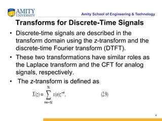
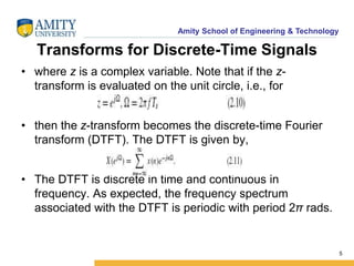
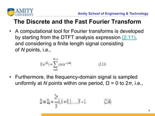
Amity School of Engineering & Technology 
1 
Amity School of Engineering & Technology 
AUDIO SIGNAL PROCESSING 
Credit Units: 4 
Mukesh Bhardwaj
Amity School of Engineering & Technology 
Module 1 
DISCRETE-TIME SIGNAL 
PROCESSING 
2
Amity School of Engineering & Technology 
DISCRETE-TIME SIGNAL PROCESSING 
• Audio coding algorithms operate on a quantized 
discrete-time signal. 
• Prior to compression, most algorithms require that the 
audio signal is acquired with high-fidelity characteristics. 
• In typical standardized algorithms, audio is assumed to 
be bandlimited at 20 kHz, sampled at 44.1 kHz, and 
quantized at 16 bits per sample. 
• In the following discussion, we will treat audio as a 
sequence, i.e., as a stream of numbers denoted 
3
Amity School of Engineering & Technology 
Transforms for Discrete-Time Signals 
• Discrete-time signals are described in the 
transform domain using the z-transform and the 
discrete-time Fourier transform (DTFT). 
• These two transformations have similar roles as 
the Laplace transform and the CFT for analog 
signals, respectively. 
• The z-transform is defined as 
4
Amity School of Engineering & Technology 
Transforms for Discrete-Time Signals 
• where z is a complex variable. Note that if the z-transform 
is evaluated on the unit circle, i.e., for 
• then the z-transform becomes the discrete-time Fourier 
transform (DTFT). The DTFT is given by, 
• The DTFT is discrete in time and continuous in 
frequency. As expected, the frequency spectrum 
associated with the DTFT is periodic with period 2π rads. 
5
Amity School of Engineering & Technology 
The Discrete and the Fast Fourier Transform 
• A computational tool for Fourier transforms is developed 
by starting from the DTFT analysis expression (2.11), 
and considering a finite length signal consisting 
of N points, i.e., 
• Furthermore, the frequency-domain signal is sampled 
uniformly at N points within one period, Ω = 0 to 2π, i.e., 
6
Amity School of Engineering & Technology 
The Discrete and the Fast Fourier Transform 
• With the sampling in the frequency domain, the Fourier 
sum of Eq. (2.13) becomes 
• It is typical in the DSP literature to replace Ωk with the 
frequency index k and hence Eq. (2.15) can be written 
as, 
• The expression in (2.16) is called the discrete Fourier 
transform (DFT). 
7
Amity School of Engineering & Technology 
The Discrete and the Fast Fourier Transform 
• Note that the sampling in the frequency domain forces 
periodicity in the time domain, i.e., x(n) = x(n + N). 
• We also have periodicity in the frequency domain, X(k) 
= X(k + N), because the signal in the time domain is also 
discrete. 
• These periodicities create circular effects when 
convolution is performed by frequency-domain 
multiplication, i.e., 
where 
8
Amity School of Engineering & Technology 
The Discrete and the Fast Fourier Transform 
• The symbol ⊗ stands for circular or periodic convolution; 
and mod N implies modulo N subtraction of indices. 
• With the proper normalization, the DFT matrix can be 
written as a unitary matrix. 
• The N-point inverse DFT (IDFT) is written as 
• The DFT transform pair is represented by the following 
notation: 
9
Amity School of Engineering & Technology 
• The DFT can be computed efficiently using the fast Fourier 
transform (FFT). 
• The FFT takes advantage of redundancies in the DFT sum by 
decimating the sequence into subsequences with even and odd 
indices. 
• It can be shown that if N is a radix-2 integer, the N-point DFT can 
be computed using a series of butterfly stages. 
• The complexity associated with the DFT algorithm is of the order 
of N2 computations. 
• In contrast, the number of computations associated with the FFT 
algorithm is roughly of the order of N log2N. 
• This is a significant reduction in computational complexity and FFTs 
are almost always used in lieu of a DFT. 
10

1 AUDIO SIGNAL PROCESSING

  • 1.
    Amity School ofEngineering & Technology 1 Amity School of Engineering & Technology AUDIO SIGNAL PROCESSING Credit Units: 4 Mukesh Bhardwaj
  • 2.
    Amity School ofEngineering & Technology Module 1 DISCRETE-TIME SIGNAL PROCESSING 2
  • 3.
    Amity School ofEngineering & Technology DISCRETE-TIME SIGNAL PROCESSING • Audio coding algorithms operate on a quantized discrete-time signal. • Prior to compression, most algorithms require that the audio signal is acquired with high-fidelity characteristics. • In typical standardized algorithms, audio is assumed to be bandlimited at 20 kHz, sampled at 44.1 kHz, and quantized at 16 bits per sample. • In the following discussion, we will treat audio as a sequence, i.e., as a stream of numbers denoted 3
  • 4.
    Amity School ofEngineering & Technology Transforms for Discrete-Time Signals • Discrete-time signals are described in the transform domain using the z-transform and the discrete-time Fourier transform (DTFT). • These two transformations have similar roles as the Laplace transform and the CFT for analog signals, respectively. • The z-transform is defined as 4
  • 5.
    Amity School ofEngineering & Technology Transforms for Discrete-Time Signals • where z is a complex variable. Note that if the z-transform is evaluated on the unit circle, i.e., for • then the z-transform becomes the discrete-time Fourier transform (DTFT). The DTFT is given by, • The DTFT is discrete in time and continuous in frequency. As expected, the frequency spectrum associated with the DTFT is periodic with period 2π rads. 5
  • 6.
    Amity School ofEngineering & Technology The Discrete and the Fast Fourier Transform • A computational tool for Fourier transforms is developed by starting from the DTFT analysis expression (2.11), and considering a finite length signal consisting of N points, i.e., • Furthermore, the frequency-domain signal is sampled uniformly at N points within one period, Ω = 0 to 2π, i.e., 6
  • 7.
    Amity School ofEngineering & Technology The Discrete and the Fast Fourier Transform • With the sampling in the frequency domain, the Fourier sum of Eq. (2.13) becomes • It is typical in the DSP literature to replace Ωk with the frequency index k and hence Eq. (2.15) can be written as, • The expression in (2.16) is called the discrete Fourier transform (DFT). 7
  • 8.
    Amity School ofEngineering & Technology The Discrete and the Fast Fourier Transform • Note that the sampling in the frequency domain forces periodicity in the time domain, i.e., x(n) = x(n + N). • We also have periodicity in the frequency domain, X(k) = X(k + N), because the signal in the time domain is also discrete. • These periodicities create circular effects when convolution is performed by frequency-domain multiplication, i.e., where 8
  • 9.
    Amity School ofEngineering & Technology The Discrete and the Fast Fourier Transform • The symbol ⊗ stands for circular or periodic convolution; and mod N implies modulo N subtraction of indices. • With the proper normalization, the DFT matrix can be written as a unitary matrix. • The N-point inverse DFT (IDFT) is written as • The DFT transform pair is represented by the following notation: 9
  • 10.
    Amity School ofEngineering & Technology • The DFT can be computed efficiently using the fast Fourier transform (FFT). • The FFT takes advantage of redundancies in the DFT sum by decimating the sequence into subsequences with even and odd indices. • It can be shown that if N is a radix-2 integer, the N-point DFT can be computed using a series of butterfly stages. • The complexity associated with the DFT algorithm is of the order of N2 computations. • In contrast, the number of computations associated with the FFT algorithm is roughly of the order of N log2N. • This is a significant reduction in computational complexity and FFTs are almost always used in lieu of a DFT. 10

Editor's Notes