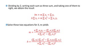
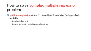
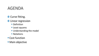
The document discusses linear regression as a key statistical and machine learning method for predictive modeling, focusing on curve fitting and least squares. It outlines the process of fitting a line to a dataset, using a training set of house prices and sizes, and minimizes errors through a cost function. Additionally, it addresses advanced topics like multiple linear regression and optimization methods such as gradient descent.

1. Linear RegressionDr. Mostafa A. Elhosseini

2. Linear Regression: Big Picture
Dr. Mostafa A. Elhosseini

3. AGENDA
Ꚛ Curve fitting.
Ꚛ Linear regression
▪ Definition
▪ Least squares
▪ Understanding the model
▪ Notations
▪ Cost function
▪ Main objective

4. Curve fitting
Ꚛ In curve fitting we are given n points (pairs of numbers) and we
want to determine a function 𝑓(𝑥) such that
▪ 𝑓 𝑥1 ≈ 𝑦1, … 𝑓 𝑥 𝑛 ≈ 𝑦𝑛
Ꚛ The type of function (for example, polynomials, exponential
functions, sine and cosine functions) may be suggested by the
nature of the problem (the underlying physical law, for instance),
and in many cases a polynomial of a certain degree will be
appropriate.

5. Linear regression
Ꚛ if the experiment values obtained in an
experiment and thus involve an
experimental error, and if the nature of
the experiment suggests a linear
relation, we better fit a straight line
through the points.
▪ Such a line may be useful for predicting
values to be expected
for other values of x

6. Linear regression
Ꚛ Linear Regression is one of the most common, some 200 years old
and most easily understandable in statistics and machine learning
▪ it comes under predictive modelling.
▪ Predictive modelling is a kind of modelling here the possible output(Y) for the
given input(X) is predicted based on the previous data or values.
Ꚛ A widely used principle for fitting straight lines is the method of
least squares by Gauss and Legendre

7. Least Squares
▪ The straight line
𝑦 = 𝑚𝑥 + 𝑏
should be fitted through the given points xi, yi , … , xn, yn so that
the sum of the squares of the distances of those points from the
straight line is minimum, where the distance is measured in the vertical
direction (the y-direction)
* Advanced Engineering Mathematics, Erwin Kreyszig, 10th edition

8. Least squares

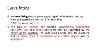
9. Understanding the model and cost function
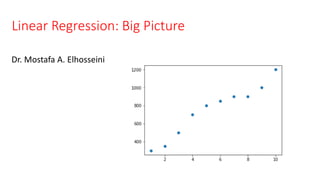
Ꚛ [Data] -- dataset that include house price and house size
Ꚛ [Training Set] -- After looking at and evaluating the data we extracted a
training set that gives us house sale prices vs house size in 𝑓𝑡2
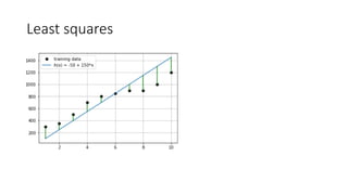
▪ Univariate linear regression
Ꚛ [Model function] -- Our model ("hypothesis" or "estimator" or
"predictor") will be a straight line "fit" to the training set".
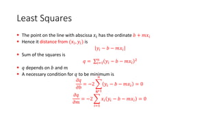
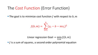
Ꚛ [Cost Function] -- Sum of squared errors that we will minimize with
respect to the model parameters.
▪ The distance between the points and line are taken and each of them is squared to
get rid of negative values and then the values are summed which gives the error
which needs to be minimized – how to minimize error?
Ꚛ [Learning Algorithm] -- Linear "least squares" Regression

10. Notation
▪ Model function ℎ 𝑥 = 𝑚𝑥 + 𝑏
▪ ℎ(𝑥) will be the price that our model predicts,
▪ ℎ(𝑥) is a function that maps house size to prices
▪ 𝑚, 𝑏 is a set of parameters for the function ℎ(𝑥) – we try to find the optimal
settings of these parameters
▪ 𝒙 is the input variable (the size of the house in square feet)
▪ 𝑦 is the selling price of the house
▪ ℎ(𝑥) is an approximation of 𝑦
▪ The subscript 𝑖 is referring to the ith data pair in out training set
▪ 𝑛 will be the number of data points

11. Datasets
▪ 𝑥 – House size from 1 𝑘𝑓𝑡2
▪ 𝑦 – Cost of the house from 300 𝐾 𝑡𝑜 1200 𝐾
▪ We have only one-factor size of the house affecting the price of the
house.
▪ In case of multiple linear regression, we would have had more factors
affecting house price like locality, the number of rooms etc

12. Main objective
The main problem in Machine Learning
▪ Find parameters for a model function that minimizes the error
between values predicted by the model and those known from the
training set.

13. Least Squares
▪ The point on the line with abscissa 𝑥𝑖 has the ordinate 𝑏 + 𝑚𝑥𝑖
▪ Hence it distance from (𝑥𝑖, 𝑦𝑖) is
𝑦𝑖 − 𝑏 − 𝑚𝑥𝑖
▪ Sum of the squares is
𝑞 = σ𝑖=1
𝑛
𝑦𝑖 − 𝑏 − 𝑚𝑥𝑖
2
▪ 𝑞 depends on 𝑏 and 𝑚
▪ A necessary condition for 𝑞 to be minimum is
𝜕𝑞
𝜕𝑏
= −2 ෍
𝑖=1
𝑛
𝑦𝑖 − 𝑏 − 𝑚𝑥𝑖 = 0
𝜕𝑞
𝜕𝑚
= −2 ෍
𝑖=1
𝑛
𝑥𝑖 𝑦𝑖 − 𝑏 − 𝑚𝑥𝑖 = 0

14. Ꚛ Dividing by 2, writing each sum as three sum, and taking one of them to
right, we obtain the result
𝑏𝑛 + 𝑚 σ 𝑥𝑖 = σ 𝑦𝑖
𝑏 σ 𝑥𝑖 + 𝑚 σ 𝑥𝑖
2
= σ 𝑥𝑖 𝑦𝑖
ꚚSolve these two equations for 𝑏, 𝑚 yields
𝑚 =
𝑛 σ𝑖 𝑥𝑖 𝑦𝑖 − (σ𝑖 𝑥𝑖)(σ𝑖 𝑦𝑖)
𝑛 σ𝑖 𝑥𝑖
2
− (σ𝑖 𝑥𝑖)2
𝑏 =
(σ𝑖 𝑦𝑖) σ𝑖 𝑥𝑖
2
− σ𝑖 𝑥𝑖 𝑦𝑖(σ𝑖 𝑥𝑖)
𝑛 σ𝑖 𝑥𝑖
2
− (σ𝑖 𝑥𝑖)2

15. The Cost Function (Error Function)
▪ The goal is to minimize cost function 𝐽 with respect to 𝑏, 𝑚
𝐽(𝑏, 𝑚) = ෍
𝑖=1
𝑛
𝑦𝑖 − 𝑏 − 𝑚𝑥𝑖
2
Linear regression Goal → min
𝑏,𝑚
𝐽(𝑏, 𝑚)
▪ 𝐽 is a sum of squares, a second order polynomial equation

16. How to solve complex multiple regression
problem
Ꚛ multiple regression refers to more than 1 predictor/independent
variable
▪ Gradient descent
▪ Heuristic-based optimization algorithm