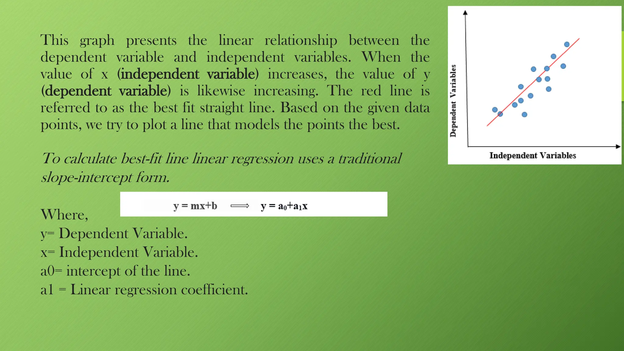
Linear Regression
Regression
It predicts the continuous output variables based on the independent input variable. like
the prediction of house prices based on different parameters like house age, distance from
the main road, location, area, etc.
1.Linear Regression
2.Polynomial Regression
3.Logistics Regression
Linear Regression
• Linear regression is a type of supervised machine learning algorithm that
computes the linear relationship between a dependent variable and one or more
independent features.
• If there is a single input variable (x), such linear regression is called simple linear
regression.
• If there is more than one input variable, such linear regression is called multiple
linear regression.
• The goal of the algorithm is to find the best linear equation that can predict the
value of the dependent variable based on the independent variables.
This graph presents the linear relationship between the
dependent variable and independent variables. When the
value of x (independent variable) increases, the value of y
(dependent variable) is likewise increasing. The red line is
referred to as the best fit straight line. Based on the given data
points, we try to plot a line that models the points the best.
To calculate best-fit line linear regression uses a traditional
slope-intercept form.
Where,
y= Dependent Variable.
x= Independent Variable.
a0= intercept of the line.
a1 = Linear regression coefficient.
A regression line can be a Positive Linear Relationship or a Negative Linear Relationship.
Positive Linear Relationship: If the dependent variable expands on the Y-axis and the
independent variable progress on X-axis, then such a relationship is termed a Positive linear
relationship.
Negative Linear Relationship: If the dependent variable decreases on the Y-axis and the
independent variable increases on the X-axis, such a relationship is called a negative linear
relationship.
The Main goal of Linear Regression
The goal of the linear regression algorithm is to get the best values for m(slope)
and c(intercept) to find the best fit line. The best fit line should have the least
error means the error between predicted values and actual values should be
minimized.
Assumption for Linear Regression Model
Linear regression is a powerful tool for understanding and predicting the behavior of a
variable, however, it needs to meet a few conditions in order to be accurate and
dependable solutions.
1.Linearity: The independent and dependent variables have a linear relationship with one
another. This implies that changes in the dependent variable follow those in the
independent variable(s) in a linear fashion.
▪ Independence: The observations in the dataset are independent of each other. This
means that the value of the dependent variable for one observation does not depend on
the value of the dependent variable for another observation.
▪ Normality: The errors in the model are normally distributed.
▪ No multicollinearity: There is no high correlation between the independent variables.
This indicates that there is little or no correlation between the independent variables.
2. Normality: The X and Y variables should be normally distributed. Histograms, KDE
plots, Q-Q plots can be used to check the Normality assumption.
3. Homoscedasticity: Across all levels of the independent
variable(s), the variance of the errors is constant. This indicates
that the amount of the independent variable(s) has no impact on
the variance of the errors.
• Equation of Simple Linear Regression, where bo is the
intercept, b1 is coefficient or slope, x is the independent
variable and y is the dependent variable.
• Equation of Multiple Linear Regression, where bo is the
intercept, b1,b2,b3,b4…,bn are coefficients or slopes of the
independent variables x1,x2,x3,x4…,xn and y is the
dependent variable.
Error is the difference between the actual value and Predicted value and the goal is to reduce this
difference.
Let’s understand this with the help of a diagram.
In the above diagram,
• x is our dependent variable which is plotted on the x-axis and y is the dependent variable which
is plotted on the y-axis.
• Black dots are the data points i.e the actual values.
• bo is the intercept which is 10 and b1 is the slope of the x variable.
• The blue line is the best fit line predicted by the model i.e the predicted values lie on the blue
line.
The vertical distance between the data point and the regression line is known as error or
residual. Each data point has one residual and the sum of all the differences is known as the Sum
of Residuals/Errors.
https://observablehq.com/@yizhe-
ang/interactive-visualization-of-linear-regression
The goal of the linear regression algorithm is to
get the best values for B0 and B1 to find the best
fit line. The best fit line is a line that has the least
error which means the error between predicted
values and actual values should be minimum.
• The cost function helps to work out the optimal values for B0 and B1, which provides
the best fit line for the data points.
• In Linear Regression, generally Mean Squared Error (MSE) cost function is used,
which is the average of squared error that occurred between the ypredicted and yi.
• We calculate MSE using simple linear equation y=mx+b:
• Using the MSE function, we’ll update the values of B0 and B1 such that the MSE
value settles at the minima. These parameters can be determined using the gradient
descent method such that the value for the cost function is minimum.
Cost Function for Linear Regression
Gradient Descent in Linear Regression
• Gradient Descent is one of the optimization algorithms that optimize the cost
function(objective function) to reach the optimal minimal solution. To find the optimum
solution we need to reduce the cost function(MSE) for all data points. This is done by
updating the values of B0 and B1 iteratively until we get an optimal solution.
• A regression model optimizes the gradient descent algorithm to update the coefficients of
the line by reducing the cost function by randomly selecting coefficient values and then
iteratively updating the values to reach the minimum cost function.
To update B0 and B1, we take gradients from the cost function. To find these gradients,
we take partial derivatives for B0 and B1.
We need to minimize the cost function J.
One of the ways to achieve this is to apply
the batch gradient descent algorithm. In
batch gradient descent, the values are
updated in each iteration. (Last two
equations shows the updating of values)
The partial derivates are the gradients, and
they are used to update the values of
B0 and B1. Alpha is the learning rate.
Evaluation Metrics for Linear Regression
• The strength of any linear regression model can be assessed using various
evaluation metrics. These evaluation metrics usually provide a measure of how
well the observed outputs are being generated by the model.
• The most used metrics are,
1. Coefficient of Determination or R-Squared (R2)
2. Root Mean Squared Error (RSME) and Residual Standard Error (RSE)
1. Coefficient of Determination or R-Squared (R2)
R-Squared is a number that explains the amount of variation that is explained/captured by the
developed model. It always ranges between 0 & 1 . Overall, the higher the value of R-squared, the
better the model fits the data.
Mathematically it can be represented as,
R2 = 1 – ( RSS/TSS )
Residual sum of Squares (RSS) is defined as the sum of squares of the residual for each data point in
the plot/data. It is the measure of the difference between the expected and the actual observed
output.
Total Sum of Squares (TSS) is defined as the sum of errors of the data points from the mean of the
response variable. Mathematically TSS is,
2. Root Mean Squared Error
• The Root Mean Squared Error is the square root of the variance of the residuals.
It specifies the absolute fit of the model to the data i.e. how close the observed
data points are to the predicted values. Mathematically it can be represented as,
• To make this estimate unbiased, one has to divide the sum of the squared
residuals by the degrees of freedom rather than the total number of data points
in the model. This term is then called the Residual Standard Error(RSE).
Mathematically it can be represented as,
Download Data set from here
https://observablehq.com/@yizhe-ang/interactive-visualization-of-linear-regression
https://scikit-learn.org/stable/modules/generated/sklearn.linear_model.LinearRegression.html
Mathematical Approach:
Residual/Error = Actual values – Predicted Values
Sum of Residuals/Errors = Sum(Actual- Predicted Values)
Square of Sum of Residuals/Errors = (Sum(Actual- Predicted Values))2
Visualization of linear regression
https://www.kaggle.com/code/ashydv/sales-prediction-simple-linear-regression/input

The normal presentation about linear regression in machine learning

  • 1.
  • 2.
    Regression It predicts thecontinuous output variables based on the independent input variable. like the prediction of house prices based on different parameters like house age, distance from the main road, location, area, etc. 1.Linear Regression 2.Polynomial Regression 3.Logistics Regression
  • 3.
    Linear Regression • Linearregression is a type of supervised machine learning algorithm that computes the linear relationship between a dependent variable and one or more independent features. • If there is a single input variable (x), such linear regression is called simple linear regression. • If there is more than one input variable, such linear regression is called multiple linear regression. • The goal of the algorithm is to find the best linear equation that can predict the value of the dependent variable based on the independent variables.
  • 4.
    This graph presentsthe linear relationship between the dependent variable and independent variables. When the value of x (independent variable) increases, the value of y (dependent variable) is likewise increasing. The red line is referred to as the best fit straight line. Based on the given data points, we try to plot a line that models the points the best. To calculate best-fit line linear regression uses a traditional slope-intercept form. Where, y= Dependent Variable. x= Independent Variable. a0= intercept of the line. a1 = Linear regression coefficient.
  • 5.
    A regression linecan be a Positive Linear Relationship or a Negative Linear Relationship. Positive Linear Relationship: If the dependent variable expands on the Y-axis and the independent variable progress on X-axis, then such a relationship is termed a Positive linear relationship. Negative Linear Relationship: If the dependent variable decreases on the Y-axis and the independent variable increases on the X-axis, such a relationship is called a negative linear relationship.
  • 6.
    The Main goalof Linear Regression The goal of the linear regression algorithm is to get the best values for m(slope) and c(intercept) to find the best fit line. The best fit line should have the least error means the error between predicted values and actual values should be minimized.
  • 7.
    Assumption for LinearRegression Model Linear regression is a powerful tool for understanding and predicting the behavior of a variable, however, it needs to meet a few conditions in order to be accurate and dependable solutions. 1.Linearity: The independent and dependent variables have a linear relationship with one another. This implies that changes in the dependent variable follow those in the independent variable(s) in a linear fashion.
  • 8.
    ▪ Independence: Theobservations in the dataset are independent of each other. This means that the value of the dependent variable for one observation does not depend on the value of the dependent variable for another observation. ▪ Normality: The errors in the model are normally distributed. ▪ No multicollinearity: There is no high correlation between the independent variables. This indicates that there is little or no correlation between the independent variables. 2. Normality: The X and Y variables should be normally distributed. Histograms, KDE plots, Q-Q plots can be used to check the Normality assumption.
  • 9.
    3. Homoscedasticity: Acrossall levels of the independent variable(s), the variance of the errors is constant. This indicates that the amount of the independent variable(s) has no impact on the variance of the errors. • Equation of Simple Linear Regression, where bo is the intercept, b1 is coefficient or slope, x is the independent variable and y is the dependent variable. • Equation of Multiple Linear Regression, where bo is the intercept, b1,b2,b3,b4…,bn are coefficients or slopes of the independent variables x1,x2,x3,x4…,xn and y is the dependent variable.
  • 10.
    Error is thedifference between the actual value and Predicted value and the goal is to reduce this difference. Let’s understand this with the help of a diagram. In the above diagram, • x is our dependent variable which is plotted on the x-axis and y is the dependent variable which is plotted on the y-axis. • Black dots are the data points i.e the actual values. • bo is the intercept which is 10 and b1 is the slope of the x variable. • The blue line is the best fit line predicted by the model i.e the predicted values lie on the blue line. The vertical distance between the data point and the regression line is known as error or residual. Each data point has one residual and the sum of all the differences is known as the Sum of Residuals/Errors. https://observablehq.com/@yizhe- ang/interactive-visualization-of-linear-regression The goal of the linear regression algorithm is to get the best values for B0 and B1 to find the best fit line. The best fit line is a line that has the least error which means the error between predicted values and actual values should be minimum.
  • 11.
    • The costfunction helps to work out the optimal values for B0 and B1, which provides the best fit line for the data points. • In Linear Regression, generally Mean Squared Error (MSE) cost function is used, which is the average of squared error that occurred between the ypredicted and yi. • We calculate MSE using simple linear equation y=mx+b: • Using the MSE function, we’ll update the values of B0 and B1 such that the MSE value settles at the minima. These parameters can be determined using the gradient descent method such that the value for the cost function is minimum. Cost Function for Linear Regression
  • 12.
    Gradient Descent inLinear Regression • Gradient Descent is one of the optimization algorithms that optimize the cost function(objective function) to reach the optimal minimal solution. To find the optimum solution we need to reduce the cost function(MSE) for all data points. This is done by updating the values of B0 and B1 iteratively until we get an optimal solution. • A regression model optimizes the gradient descent algorithm to update the coefficients of the line by reducing the cost function by randomly selecting coefficient values and then iteratively updating the values to reach the minimum cost function.
  • 13.
    To update B0and B1, we take gradients from the cost function. To find these gradients, we take partial derivatives for B0 and B1.
  • 14.
    We need tominimize the cost function J. One of the ways to achieve this is to apply the batch gradient descent algorithm. In batch gradient descent, the values are updated in each iteration. (Last two equations shows the updating of values) The partial derivates are the gradients, and they are used to update the values of B0 and B1. Alpha is the learning rate.
  • 15.
    Evaluation Metrics forLinear Regression • The strength of any linear regression model can be assessed using various evaluation metrics. These evaluation metrics usually provide a measure of how well the observed outputs are being generated by the model. • The most used metrics are, 1. Coefficient of Determination or R-Squared (R2) 2. Root Mean Squared Error (RSME) and Residual Standard Error (RSE)
  • 16.
    1. Coefficient ofDetermination or R-Squared (R2) R-Squared is a number that explains the amount of variation that is explained/captured by the developed model. It always ranges between 0 & 1 . Overall, the higher the value of R-squared, the better the model fits the data. Mathematically it can be represented as, R2 = 1 – ( RSS/TSS ) Residual sum of Squares (RSS) is defined as the sum of squares of the residual for each data point in the plot/data. It is the measure of the difference between the expected and the actual observed output. Total Sum of Squares (TSS) is defined as the sum of errors of the data points from the mean of the response variable. Mathematically TSS is,
  • 17.
    2. Root MeanSquared Error • The Root Mean Squared Error is the square root of the variance of the residuals. It specifies the absolute fit of the model to the data i.e. how close the observed data points are to the predicted values. Mathematically it can be represented as, • To make this estimate unbiased, one has to divide the sum of the squared residuals by the degrees of freedom rather than the total number of data points in the model. This term is then called the Residual Standard Error(RSE). Mathematically it can be represented as,
  • 19.
    Download Data setfrom here https://observablehq.com/@yizhe-ang/interactive-visualization-of-linear-regression https://scikit-learn.org/stable/modules/generated/sklearn.linear_model.LinearRegression.html Mathematical Approach: Residual/Error = Actual values – Predicted Values Sum of Residuals/Errors = Sum(Actual- Predicted Values) Square of Sum of Residuals/Errors = (Sum(Actual- Predicted Values))2 Visualization of linear regression https://www.kaggle.com/code/ashydv/sales-prediction-simple-linear-regression/input