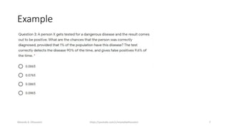
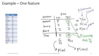
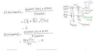
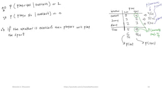
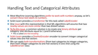
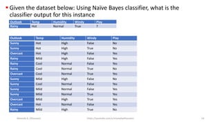
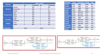
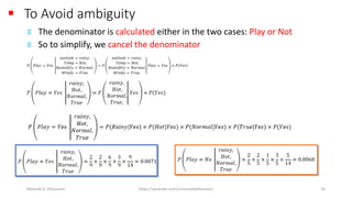
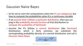
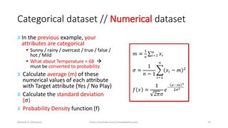
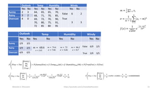
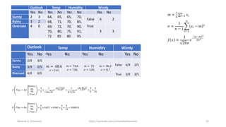
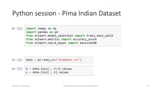
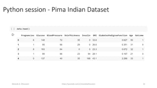
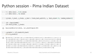
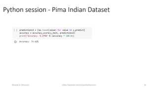
Naive bayes classifier python session

Naïve Bayes’ Classifier
Python Session
Dr. Mostafa A. Elhosseini

Agenda
≡Naïve Bayes’s Theorem
▪ Examples test have a disease
≡Python session
▪ Example
▪ Categorical features
▪ Continues variable - Non categorical attribute
Mostafa A. Elhosseini https://youtube.com/c/mostafaelhosseini 2

Example: Bayes’s Theorem
≡ Suppose a certain disease has an incidence rate of 0.1% (that is, it
afflicts 0.1% of the population). A test has been devised to detect this
disease. The test does not produce false negatives (that is, anyone
who has the disease will test positive for it), but the false positive
rate is 5% (that is, about 5% of people who take the test will test
positive, even though they do not have the disease).
≡ Suppose a randomly selected person takes the test and tests positive.
What is the probability that this person actually has the disease?

≡ The disease has an incidence rate of 0.1%, we could write P(disease)
= 0.001
≡ Everyone who has the disease will test positive, or alternatively
everyone who tests negative does not have the disease. (We could
also say P(positive | disease) = 1.)
≡ about 5% of people who take the test will test positive, even though
they do not have the disease P(positive | no disease) = 0.05.)
≡ Here we want to compute P(disease|positive)

≡ First, suppose we randomly select 1000 people and administer the test
≡ Only 1 of 1000 test subjects actually has the disease; the other 999 do not.
≡ We also know that 5% of all people who do not have the disease will test
positive. There are 999 disease-free people, so we would expect
(0.05)(999) = 49.95 (so, about 50) people to test positive who do not have
the disease.
≡ There are 51 people who test positive in our example (the one
unfortunate person who actually has the disease, plus the 50 people who
tested positive but don’t). Only one of these people has the disease, so
≡ P(disease | positive) ≈ 1/51≈ 0.0196, or less than 2%.
≡ This means that of all people who test positive, over 98% do not have the
disease.

≡ 𝑝 𝑑𝑖𝑠𝑒𝑎𝑠𝑒 𝑝𝑜𝑠𝑖𝑖𝑣𝑒 =
𝑝(𝑝𝑜𝑠𝑖𝑡𝑖𝑣𝑒|𝑑𝑖𝑠𝑒𝑎𝑠𝑒)𝑝 𝑑𝑖𝑠𝑒𝑎𝑠𝑒
𝑝 𝑝𝑜𝑠𝑖𝑡𝑖𝑣𝑒 𝑑𝑖𝑠𝑒𝑎𝑠𝑒 𝑝 𝑑𝑖𝑠𝑒𝑎𝑠𝑒 +𝑝 𝑝𝑜𝑠𝑖𝑡𝑖𝑣𝑒 𝑛𝑜 𝑑𝑖𝑠𝑒𝑎𝑠𝑒 𝑝 𝑛𝑜 𝑑𝑖𝑠𝑒𝑎𝑠𝑒
≡ 𝑝 𝑑𝑖𝑠𝑒𝑎𝑠𝑒 𝑝𝑜𝑠𝑖𝑖𝑣𝑒 =
1×0.001
1×0.001+0.05∗0.999
= 0.0196

Example

Example – One feature

Handling Text and Categorical Attributes
Ꚛ Most Machine Learning algorithms prefer to work with numbers anyway, so let’s
convert these text labels to numbers.
Ꚛ Scikit-Learn provides a transformer for this task called LabelEncoder
Ꚛ One issue with this representation is that ML algorithms will assume that two
nearby values are more similar than two distant values
Ꚛ To fix this issue, a common solution is to create one binary attribute per
category: one attribute equal to 1 (and 0 otherwise)
▪ This is called one-hot encoding
Ꚛ Scikit-Learn provides a OneHotEncoder encoder to convert integer categorical
values into one-hot vectors
Ꚛ We can apply both transformations (from text categories to integer categories,
then from integer categories to one-hot vectors) in one shot using the
LabelBinarizer class

Custom Transformers
Ꚛ Although Scikit-Learn provides many useful transformers, you will need to
write your own for tasks such as custom cleanup operations or combining
specific attributes.
Ꚛ You will want your transformer to work seamlessly with Scikit-Learn
functionalities (such as pipelines)
Ꚛ hyperparameter will allow you to easily find out whether adding this
attribute helps the Machine Learning algorithms or not.
Ꚛ More generally, you can add a hyperparameter to gate any data
preparation step that you are not 100% sure about.
Ꚛ The more you automate these data preparation steps, the more
combinations you can automatically try out, making it much more likely
that you will find a great combination (and saving you a lot of time).

Python
https://colab.research.google.com/drive/1tu3_CWRnl9aylppme0s4cN9-M3w6nj7F#scrollTo=il4fDyb7vcwr

▪ Given the dataset below: Using Naïve Bayes classifier, what is the
classifier output for this instance
Outlook Temp Humidity Windy Play
Rainy Hot Normal True ?
Sunny Hot High False No
Sunny Hot High True No
Overcast Hot High False Yes
Rainy Mild High False Yes
Rainy Cool Normal False Yes
Rainy Cool Normal True No
Overcast Cool Normal True Yes
Sunny Mild High False No
Sunny Cool Normal False Yes
Sunny Mild Normal False Yes
Sunny Mild Normal True Yes
Overcast Mild High True Yes
Overcast Hot Normal False Yes
Rainy Mild High True No

Feature
Play or Not?
Yes Probability No Probability
Outlook
Sunny 3 3/9 3 3/5
Overcast 4 4/9 0 0
Rainy 2 2/9 2 2/5
Temperature
Hot 2 2/9 2 2/5
Mild 4 4/9 2 2/5
Cool 3 3/9 1 1/5
Humidity
High 3 3/9 4 4/5
Normal 6 6/9 1 1/5
Windy
True 3 3/9 3 3/5
False 6 6/9 2 2/5
Probability 9/14 5/14
Sunny Hot High False No
Sunny Hot High True No
Overcast Hot High False Yes
Rainy Mild High False Yes
Rainy Cool Normal False Yes
Rainy Cool Normal True No
Overcast Cool Normal True Yes
Sunny Mild High False No
Sunny Cool Normal False Yes
Sunny Mild Normal False Yes
Sunny Mild Normal True Yes
Overcast Mild High True Yes
Overcast Hot Normal False Yes
Rainy Mild High True No

▪ To Avoid ambiguity
≡ The denominator is calculated either in the two cases: Play or Not
≡ So to simplify, we cancel the denominator

Python
https://colab.research.google.com/drive/1nVJYqUvwXVuXfmFZiAFJYTUTebXgQ17G

▪ What is the probability that instance with these attributes is classified
as Play
Sunny 66 99 True ?

Gaussian Naïve Bayes
≡ So far we’ve seen the computations when the X’s are categorical, but
how to compute the probabilities when X is a continuous variable
≡ If we assume that x follows a particular distribution, then you can
plug in the probability density function of that distribution to
compute the probability of likelihoods
≡ Assume the X’s follows a normal distribution (aka Gaussian)
Distribution, which is fairly common, we substitute the
corresponding probability density of a normal distribution and call it
Gaussian Naïve Bayes
𝑓 𝑥 =
1
2𝜋𝜎
𝑒
−
𝑥−𝑚 2
2𝜎2

Categorical dataset // Numerical dataset
≡ In the previous example, your
attributes are categorical
▪ Sunny / rainy / overcast / true / false /
hot / Mild
▪ What about Temperature = 68 →
must be converted to probability
≡ Calculate average (m) of these
numerical values of each attribute
with Target attribute (Yes / No Play)
≡ Calculate the standard deviation
(𝜎)
≡ Probability Density function (f)

Outlook Temp Humidity Windy
Yes No Yes No Yes No Yes No
Sunny 2 3 64,
68,
69,
70,
72
65,
71,
72,
80,
85
65,
70,
70,
75,
80
70,
85,
90,
91,
95
False 6 2
Rainy 3 2
Overcast 4 0 True
3 3
Sunny 2/9 3/5
𝑚 = 68.6
𝜎 = 2.65
𝑚 = 74.6
𝜎 = 7.06
𝑚 = 72
𝜎 = 5.06
𝑚 = 86.2
𝜎 = 8.7
False 6/9 2/5
Rainy 3/9 2/5
Overcast 4/9 0/5 True 3/9 3/5

Sunny 2 3 64,
68,
69,
70,
72
65,
71,
72,
80,
85
65,
70,
70,
75,
80
70,
85,
90,
91,
95
False 6 2
Rainy 3 2
Overcast 4 0 True
3 3
Sunny 2/9 3/5
𝑚 = 68.6
𝜎 = 2.65
𝑚 = 74.6
𝜎 = 7.06
𝑚 = 72
𝜎 = 5.06
𝑚 = 86.2
𝜎 = 8.7
False 6/9 2/5
Rainy 3/9 2/5
Overcast 4/9 0/5 True 3/9 3/5

Example: only continuous variables

Python session
https://colab.research.google.com/drive/1FaBhZXjvu9rFhv2_sZm0lgauXa4TnSsi

Pima Indian Dataset
≡ This dataset is originally from the National Institute of Diabetes and
Digestive and Kidney Diseases.
≡ The objective of the dataset is to diagnostically predict whether or not a
patient has diabetes, based on certain diagnostic measurements included
in the dataset.
≡ Several constraints were placed on the selection of these instances from a
larger database. In particular, all patients here are females at least 21 years
old of Pima Indian heritage.
≡ The datasets consists of several medical predictor variables and one target
variable, Outcome. Predictor variables includes the number of
pregnancies the patient has had, their BMI, insulin level, age, and so on.

Pima Indian Dataset
≡ This dataset is originally from the National Institute of Diabetes and
Digestive and Kidney Diseases.
≡ BloodPressure: Diastolic blood pressure (mm Hg)
≡ SkinThicknessTriceps: skin fold thickness (mm)
≡ Insulin: 2-Hour serum insulin (mu U/ml)
≡ BMI: Body mass index (weight in kg/(height in m)^2)
≡ DiabetesPedigreeFunction: Diabetes pedigree function
≡ Age: Age (years)
≡ OutcomeClass variable (0 or 1) 268 of 768 are 1, the others are 0
≡ https://www.kaggle.com/uciml/pima-indians-diabetes-database

Pima Indian Dataset

Python session - Pima Indian Dataset

https://colab.research.google.com/drive/1AE4N6OH95Gp235V_7qiSh2Oad79g0Ixo

Naive bayes classifier python session

More Related Content

Similar to Naive bayes classifier python session

More from Mostafa El-Hosseini

Recently uploaded

Naive bayes classifier python session