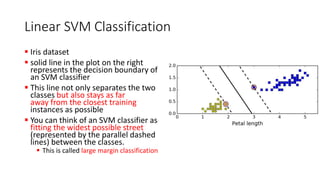
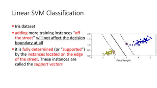
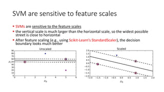
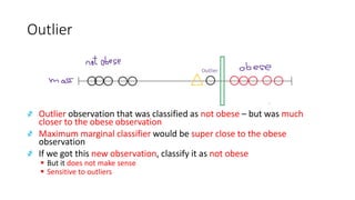
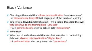
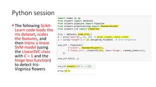
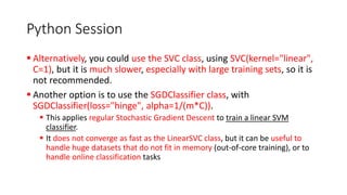
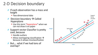
Support Vector ClassifierDr. Mostafa A. Elhosseini
YouTube Channel
StatQuest with Josh Starmer
https://www.youtube.com/watch?v=efR1C6CvhmE&list=LLZ0o2
yS-zpxZ75dVEhq_AjQ&index=6&t=0s
Lecture 1:Support Vector Machines, Clearly Explained!!!
Lecture 2: Support Vector Machines Part 2: The Polynomial
Kernel
Lecture 3: Support Vector Machines Part 3: The Radial (RBF)
Kernel
THE BIAS/VARIANCE TRADEOFF
≡model’s generalization error can be expressed as the sum of three
very different errors:
▪ Bias : This part of the generalization error is due to wrong assumptions, such
as assuming that the data is linear when it is actually quadratic. A high-bias
model is most likely to underfit the training data
▪ Variance: This part is due to the model’s excessive sensitivity to small
variations in the training data. A model with many degrees of freedom (such
as a high-degree polynomial model) is likely to have high variance, and thus to
overfit the training data.
▪ Irreducible error: This part is due to the noisiness of the data itself. The only
way to reduce this part of the error is to clean up the data (e.g., fix the data
sources, such as broken sensors, or detect and remove outliers)
THE BIAS/VARIANCE TRADEOFF
≡ Increasing a model’s complexity will typically
▪ increase its variance and
▪ reduce its bias.
≡ Conversely, reducing a model’s complexity
▪ increases its bias and
▪ reduces its variance.
≡ This is why it is called a tradeoff
▪ Intro…
≡ the linear regression is not
a great model
▪ This is underfitting
▪ Known as high bias
▪ Bias: we have a strong
preconception that there
should be a linear fit
≡ Quadratic function
▪ Works well
▪ Just right
≡ High order polynomial
▪ Perform perfect on training
data
▪ high variance
▪ Not able to generalize on
unseen data
▪ If we have too many features
𝑦 = 𝜃0 + 𝜃1 𝑥 𝑦 = 𝜃0 + 𝜃1 𝑥 + 𝜃2 𝑥2 𝑦 = 𝜃0 + 𝜃1 𝑥 + 𝜃2 𝑥2 +
𝜃3 𝑥3
+ 𝜃4 𝑥4
Cross validation
≡ As we saw earlier, you don’t want to touch the test set until you are ready
to launch a model you are confident about, so you need to use part of the
training set for training, and part for model validation
≡ Scikit-Learn provide us with cross-validation feature.
▪ It randomly splits the training set into 10 distinct subsets called folds,
▪ Then it trains and evaluates the Decision Tree model 10 times, picking a different fold
for evaluation every time and training on the other 9 folds.
▪ The result is an array containing the 10 evaluation scores
≡ If a model performs well on the training data but generalizes poorly
according to the cross-validation metrics, then your model is overfitting.
≡ If it performs poorly on both, then it is underfitting. This is one way to tell
when a model is too simple or too complex
Classification of mice mass
҂ According to mass observations:
▪ Obese or Not obese
҂ When you have a new observation “Unknown” that has less mass than threshold
▪ Classify it as not obese
҂ When it has more mass than threshold
▪ Classify it as obese
Classification of mice mass
҂ According to mass observations:
▪ Obese or Not obese
҂ When you have a new observation “Unknown” that has less mass than threshold
▪ Classify it as not obese
҂ When it has more mass than threshold
▪ Classify it as obese
Classification of mice mass
҂ If we have a new observation that has more mass than threshold
▪ We classify it as Obese
҂ But that does not make sense
▪ Because it is much closer to the observations that are not obese
҂ Threshold is pretty lame
To make it better
▪ Focus on the observation on the edges of each class
▪ Take the threshold as the midpoint between them as new threshold
▪ If a new observation comes that has low mass
▪ It will be closer to the observation that are not obese than it is to the
obese observation
▪ So it makes sense to classify this new observation as not obese
҂ Shortest distance between the observation and threshold is called
Margin
҂ Maximum Marginal Classifier:
▪ when we use the threshold that gives us the largest margin to make
classification
Support Vector Machine
҂ Support Vector Machine (SVM) is a very powerful and versatile
Machine Learning model, capable of performing linear or nonlinear
classification, regression, and even outlier detection
҂ SVMs are particularly well suited for classification of complex but
small- or medium-sized datasets
Linear SVM Classification
▪ Iris dataset
▪ The two classes can clearly be
separated easily with a straight line
(they are linearly separable)
▪ Dashed line is so bad that it does not
even separate the classes properly
▪ The other two models work perfectly
on this training set, but their decision
boundaries come so close to the
instances that these models will
probably not perform as well on new
instances
Linear SVM Classification
▪ Iris dataset
▪ solid line in the plot on the right
represents the decision boundary of
an SVM classifier
▪ This line not only separates the two
classes but also stays as far
away from the closest training
instances as possible
▪ You can think of an SVM classifier as
fitting the widest possible street
(represented by the parallel dashed
lines) between the classes.
▪ This is called large margin classification
Linear SVM Classification
▪ Iris dataset
▪ adding more training instances “off
the street” will not affect the decision
boundary at all
▪ it is fully determined (or “supported”)
by the instances located on the edge
of the street. These instances are
called the support vectors
SVM are sensitive to feature scales
▪ SVMs are sensitive to the feature scales
▪ the vertical scale is much larger than the horizontal scale, so the widest possible
street is close to horizontal
▪ After feature scaling (e.g., using Scikit-Learn’s StandardScaler), the decision
boundary looks much better
Outlier
҂ Outlier observation that was classified as not obese – but was much
closer to the obese observation
҂ Maximum marginal classifier would be super close to the obese
observation
҂ If we got this new observation, classify it as not obese
▪ But it does not make sense
▪ Sensitive to outliers
Hard margin classification
» If we strictly impose that all instances be off the street and on the right
side,
▪ this is called hard margin classification.
» There are two main issues with hard margin classification.
▪ First, it only works if the data is linearly separable, and
▪ second it is quite sensitive to outliers
» on the left, it is impossible to find a hard margin, and on the right the
decision boundary ends up very different from the one we saw without
the outlier, and it will probably not generalize as well
Soft Margin Classification
• To avoid these issues it is preferable to use a more flexible model
• The objective is to find a good balance between keeping the street as
large as possible and limiting the margin violations
• Violation: Instances that end up in the middle of the street or even on the
wrong side).
• This is called soft margin classification
• In Scikit-Learn’s SVM classes, you can control this balance using the C
hyperparameter: a smaller C value leads to a wider street but more
margin violations
To make it better
҂ To make a threshold that is not so sensitive to outliers, we must
allow misclassification
▪ Ignore outliers
▪ Put the threshold as the midpoint
▪ Misclassify this observation “Outlier”
▪ When we get a new observation, classify it as obese
▪ Makes sense
Soft Margin Classification
▪ On the left, using a high C value the classifier makes fewer margin
violations but ends up with a smaller margin.
▪ On the right, using a low C value the margin is much larger, but many
instances end up on the street.
▪ However, it seems likely that the second classifier will generalize better:
▪ in fact even on this training set it makes fewer prediction errors, since most of the
margin violations are actually on the correct side of the decision boundary
▪ If your SVM model is overfitting, you can try regularizing it by reducing C
Support Vector Classifier
• Use a soft margin to determine the location of a threshold
• Names comes from observations on the edges and within the soft
margin are called support vector
Bias / Variance
҂ Choosing a threshold that allows misclassification is an example of
the bias/variance tradeoff that plagues all of the machine learning
҂ Before we allowed misclassification – we picked a threshold that was
very sensitive to the training data “Low Bias”
▪ As it performed poorly when we got new data “High variance”
҂ In contrast
҂ When we picked a threshold that was less sensitive to the training
data and allowed misclassification “Higher bias”
▪ It performed better when we got new data “Low variance”
▪ Soft Margin
҂ When we allow misclassification, the distance between the observations and the
threshold is called a soft margin
Question:
҂ How do we know that this soft margin is better than this soft margin
҂ Use cross validation to determine how many misclassification and observations
to allow inside the soft margin to get the best classification
▪ Cross Validation
҂ If cross validation determined that this was the best soft margin
▪ Allow one misclassification
▪ two observations, that are correctly classified, to be within the soft margin
҂ When we use a soft margin to determine the location of a threshold, then
we are using a soft margin classifier aka Support Vector Classifier
Python session
▪ The following Scikit-
Learn code loads the
iris dataset, scales
the features, and
then trains a linear
SVM model (using
the LinearSVC class
with C = 1 and the
hinge loss function)
to detect Iris-
Virginica flowers
Python Session
▪ Alternatively, you could use the SVC class, using SVC(kernel="linear",
C=1), but it is much slower, especially with large training sets, so it is
not recommended.
▪ Another option is to use the SGDClassifier class, with
SGDClassifier(loss="hinge", alpha=1/(m*C)).
▪ This applies regular Stochastic Gradient Descent to train a linear SVM
classifier.
▪ It does not converge as fast as the LinearSVC class, but it can be useful to
handle huge datasets that do not fit in memory (out-of-core training), or to
handle online classification tasks
2-D Decision boundary
҂ If each observation has a mass and
height
▪ Two-dimensional data
҂ Decision boundary → Called
Hyperplane
▪ Use this term “Hyperplane” when we
can not draw it on paper
҂ Support vector Classifier is pretty
cool, because
▪ Handle outliers
▪ Allow overlapping classification →
because it allows misclassification
҂ But,… what if we had tons of
overlap?

Lecture 23 support vector classifier

  • 1.
    Support Vector ClassifierDr.Mostafa A. Elhosseini
  • 2.
    YouTube Channel StatQuest withJosh Starmer https://www.youtube.com/watch?v=efR1C6CvhmE&list=LLZ0o2 yS-zpxZ75dVEhq_AjQ&index=6&t=0s Lecture 1:Support Vector Machines, Clearly Explained!!! Lecture 2: Support Vector Machines Part 2: The Polynomial Kernel Lecture 3: Support Vector Machines Part 3: The Radial (RBF) Kernel
  • 3.
    THE BIAS/VARIANCE TRADEOFF ≡model’sgeneralization error can be expressed as the sum of three very different errors: ▪ Bias : This part of the generalization error is due to wrong assumptions, such as assuming that the data is linear when it is actually quadratic. A high-bias model is most likely to underfit the training data ▪ Variance: This part is due to the model’s excessive sensitivity to small variations in the training data. A model with many degrees of freedom (such as a high-degree polynomial model) is likely to have high variance, and thus to overfit the training data. ▪ Irreducible error: This part is due to the noisiness of the data itself. The only way to reduce this part of the error is to clean up the data (e.g., fix the data sources, such as broken sensors, or detect and remove outliers)
  • 4.
    THE BIAS/VARIANCE TRADEOFF ≡Increasing a model’s complexity will typically ▪ increase its variance and ▪ reduce its bias. ≡ Conversely, reducing a model’s complexity ▪ increases its bias and ▪ reduces its variance. ≡ This is why it is called a tradeoff
  • 5.
    ▪ Intro… ≡ thelinear regression is not a great model ▪ This is underfitting ▪ Known as high bias ▪ Bias: we have a strong preconception that there should be a linear fit ≡ Quadratic function ▪ Works well ▪ Just right ≡ High order polynomial ▪ Perform perfect on training data ▪ high variance ▪ Not able to generalize on unseen data ▪ If we have too many features 𝑦 = 𝜃0 + 𝜃1 𝑥 𝑦 = 𝜃0 + 𝜃1 𝑥 + 𝜃2 𝑥2 𝑦 = 𝜃0 + 𝜃1 𝑥 + 𝜃2 𝑥2 + 𝜃3 𝑥3 + 𝜃4 𝑥4
  • 6.
    Cross validation ≡ Aswe saw earlier, you don’t want to touch the test set until you are ready to launch a model you are confident about, so you need to use part of the training set for training, and part for model validation ≡ Scikit-Learn provide us with cross-validation feature. ▪ It randomly splits the training set into 10 distinct subsets called folds, ▪ Then it trains and evaluates the Decision Tree model 10 times, picking a different fold for evaluation every time and training on the other 9 folds. ▪ The result is an array containing the 10 evaluation scores ≡ If a model performs well on the training data but generalizes poorly according to the cross-validation metrics, then your model is overfitting. ≡ If it performs poorly on both, then it is underfitting. This is one way to tell when a model is too simple or too complex
  • 7.
    Classification of micemass ҂ According to mass observations: ▪ Obese or Not obese ҂ When you have a new observation “Unknown” that has less mass than threshold ▪ Classify it as not obese ҂ When it has more mass than threshold ▪ Classify it as obese
  • 8.
    Classification of micemass ҂ According to mass observations: ▪ Obese or Not obese ҂ When you have a new observation “Unknown” that has less mass than threshold ▪ Classify it as not obese ҂ When it has more mass than threshold ▪ Classify it as obese
  • 9.
    Classification of micemass ҂ If we have a new observation that has more mass than threshold ▪ We classify it as Obese ҂ But that does not make sense ▪ Because it is much closer to the observations that are not obese ҂ Threshold is pretty lame
  • 10.
    To make itbetter ▪ Focus on the observation on the edges of each class ▪ Take the threshold as the midpoint between them as new threshold
  • 11.
    ▪ If anew observation comes that has low mass ▪ It will be closer to the observation that are not obese than it is to the obese observation ▪ So it makes sense to classify this new observation as not obese
  • 12.
    ҂ Shortest distancebetween the observation and threshold is called Margin ҂ Maximum Marginal Classifier: ▪ when we use the threshold that gives us the largest margin to make classification
  • 13.
    Support Vector Machine ҂Support Vector Machine (SVM) is a very powerful and versatile Machine Learning model, capable of performing linear or nonlinear classification, regression, and even outlier detection ҂ SVMs are particularly well suited for classification of complex but small- or medium-sized datasets
  • 14.
    Linear SVM Classification ▪Iris dataset ▪ The two classes can clearly be separated easily with a straight line (they are linearly separable) ▪ Dashed line is so bad that it does not even separate the classes properly ▪ The other two models work perfectly on this training set, but their decision boundaries come so close to the instances that these models will probably not perform as well on new instances
  • 15.
    Linear SVM Classification ▪Iris dataset ▪ solid line in the plot on the right represents the decision boundary of an SVM classifier ▪ This line not only separates the two classes but also stays as far away from the closest training instances as possible ▪ You can think of an SVM classifier as fitting the widest possible street (represented by the parallel dashed lines) between the classes. ▪ This is called large margin classification
  • 16.
    Linear SVM Classification ▪Iris dataset ▪ adding more training instances “off the street” will not affect the decision boundary at all ▪ it is fully determined (or “supported”) by the instances located on the edge of the street. These instances are called the support vectors
  • 17.
    SVM are sensitiveto feature scales ▪ SVMs are sensitive to the feature scales ▪ the vertical scale is much larger than the horizontal scale, so the widest possible street is close to horizontal ▪ After feature scaling (e.g., using Scikit-Learn’s StandardScaler), the decision boundary looks much better
  • 18.
    Outlier ҂ Outlier observationthat was classified as not obese – but was much closer to the obese observation ҂ Maximum marginal classifier would be super close to the obese observation ҂ If we got this new observation, classify it as not obese ▪ But it does not make sense ▪ Sensitive to outliers
  • 19.
    Hard margin classification »If we strictly impose that all instances be off the street and on the right side, ▪ this is called hard margin classification. » There are two main issues with hard margin classification. ▪ First, it only works if the data is linearly separable, and ▪ second it is quite sensitive to outliers » on the left, it is impossible to find a hard margin, and on the right the decision boundary ends up very different from the one we saw without the outlier, and it will probably not generalize as well
  • 20.
    Soft Margin Classification •To avoid these issues it is preferable to use a more flexible model • The objective is to find a good balance between keeping the street as large as possible and limiting the margin violations • Violation: Instances that end up in the middle of the street or even on the wrong side). • This is called soft margin classification • In Scikit-Learn’s SVM classes, you can control this balance using the C hyperparameter: a smaller C value leads to a wider street but more margin violations
  • 21.
    To make itbetter ҂ To make a threshold that is not so sensitive to outliers, we must allow misclassification ▪ Ignore outliers ▪ Put the threshold as the midpoint ▪ Misclassify this observation “Outlier” ▪ When we get a new observation, classify it as obese ▪ Makes sense
  • 22.
    Soft Margin Classification ▪On the left, using a high C value the classifier makes fewer margin violations but ends up with a smaller margin. ▪ On the right, using a low C value the margin is much larger, but many instances end up on the street. ▪ However, it seems likely that the second classifier will generalize better: ▪ in fact even on this training set it makes fewer prediction errors, since most of the margin violations are actually on the correct side of the decision boundary ▪ If your SVM model is overfitting, you can try regularizing it by reducing C
  • 23.
    Support Vector Classifier •Use a soft margin to determine the location of a threshold • Names comes from observations on the edges and within the soft margin are called support vector
  • 24.
    Bias / Variance ҂Choosing a threshold that allows misclassification is an example of the bias/variance tradeoff that plagues all of the machine learning ҂ Before we allowed misclassification – we picked a threshold that was very sensitive to the training data “Low Bias” ▪ As it performed poorly when we got new data “High variance” ҂ In contrast ҂ When we picked a threshold that was less sensitive to the training data and allowed misclassification “Higher bias” ▪ It performed better when we got new data “Low variance”
  • 25.
    ▪ Soft Margin ҂When we allow misclassification, the distance between the observations and the threshold is called a soft margin Question: ҂ How do we know that this soft margin is better than this soft margin ҂ Use cross validation to determine how many misclassification and observations to allow inside the soft margin to get the best classification
  • 26.
    ▪ Cross Validation ҂If cross validation determined that this was the best soft margin ▪ Allow one misclassification ▪ two observations, that are correctly classified, to be within the soft margin ҂ When we use a soft margin to determine the location of a threshold, then we are using a soft margin classifier aka Support Vector Classifier
  • 27.
    Python session ▪ Thefollowing Scikit- Learn code loads the iris dataset, scales the features, and then trains a linear SVM model (using the LinearSVC class with C = 1 and the hinge loss function) to detect Iris- Virginica flowers
  • 28.
    Python Session ▪ Alternatively,you could use the SVC class, using SVC(kernel="linear", C=1), but it is much slower, especially with large training sets, so it is not recommended. ▪ Another option is to use the SGDClassifier class, with SGDClassifier(loss="hinge", alpha=1/(m*C)). ▪ This applies regular Stochastic Gradient Descent to train a linear SVM classifier. ▪ It does not converge as fast as the LinearSVC class, but it can be useful to handle huge datasets that do not fit in memory (out-of-core training), or to handle online classification tasks
  • 29.
    2-D Decision boundary ҂If each observation has a mass and height ▪ Two-dimensional data ҂ Decision boundary → Called Hyperplane ▪ Use this term “Hyperplane” when we can not draw it on paper ҂ Support vector Classifier is pretty cool, because ▪ Handle outliers ▪ Allow overlapping classification → because it allows misclassification ҂ But,… what if we had tons of overlap?