This is best ppt

1. Introduction to
Linear
Regression
Understanding the Basics and Applications
Presented by:Kevin mathukiya
Roll no :

2. Agenda
• Introduction to Linear Regression
• Importance and Types of Linear
Regression
• Key Concepts
• Mathematical Formulas
• Best Fit Line and Cost Function
• Gradient Descent
• Steps to Perform Linear Regression
• Evaluating Model Performance
• Applications of Linear Regression
• Practice Example with Code
• Advantages and Disadvantages
• Bibliography

3. What is Linear
Regression?
• Definition: Linear Regression is a
statistical method to model the
relationship between a dependent
variable and one or more
independent variables.
• Purpose: To predict the value of the
dependent variable based on the
values of independent variables.

4. Importance of Linear
Regression
•Simple Prediction: Linear regression
predicts outcomes based on input
data using a straightforward
mathematical formula.
•Wide Applicability: It's used in
science, business, and various other
fields due to its versatility.
•Reliability: Linear regression provides
reliable predictions and is quick to
train due to its well-understood
properties.

5. Key concepts
• Dependent Variable (Y): The outcome
we are trying to predict.​
• Independent Variable (X): The
predictor or explanatory variable.​
• Linear Relationship: Assumes a
straight-line relationship between X
and Y.​
• Regression Line: The line that best fits
the data points.

6. Types of Linear
Regression
•Simple Linear Regression: Involves one
independent
variable and predicts a continuous outcome.
•Multiple Linear Regression: Includes multiple
independent variables to predict a continuous
outcome.
•Polynomial Regression: Fits a curve to data by
including polynomial terms in the regression
equation.

7. Mathematical Formulas
• Simple Linear Regression:
• y = ß0 + ß1X
• Multiple Linear Regression:
• y = ß0 + ß1X1 + ß2X2 + ... + ßnXn
• Key terms:
• - y: Dependent variable
• - X: Independent variable(s)
• - ß0: Intercept
• - ß1, ß2, ... , ßn: Slopes

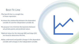
8. Best Fit Line
•The best-fit line is a straight line
in linear regression.
•It shows the relationship between the dependent
variable (Y) and the independent variable (X).
•Its purpose is to minimize discrepancies between
actual data points and predicted values.
•Optimal values for the intercept (β0) and slope (β1)
are found to determine this line.
•Helps understand and predict changes in the dependent
variable with changes in the independent variable.

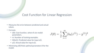
9. Cost Function for Linear Regression
• Measures the error between predicted and actual
values.
• Formula:
• J(θ): Cost function, where θ are model
parameters.
• m: Number of training examples.
• hθ​
(x(i)): Predicted value for input x(i).
• y(i): Actual value for input x(i).
• Minimizing J(θ) finds optimal parameters θ for the
model.

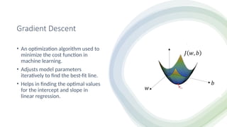
10. Gradient Descent
• An optimization algorithm used to
minimize the cost function in
machine learning.
• Adjusts model parameters
iteratively to find the best-fit line.
• Helps in finding the optimal values
for the intercept and slope in
linear regression.

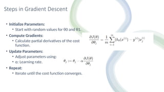
11. Steps in Gradient Descent
• Initialize Parameters:
• Start with random values for θ0​and θ1.
• Compute Gradients:
• Calculate partial derivatives of the cost
function.
• Update Parameters:
• Adjust parameters using:
• α: Learning rate.
• Repeat:
• Iterate until the cost function converges.

12. Steps to Perform
Linear
Regression
1. Data Collection: Gather data for
dependent and independent variables.
2. Data Preprocessing: Clean and prepare
the data.
3. Model Training: Fit the linear regression
model to the data.
4. Model Testing: Evaluate the model using
test data.
5. Prediction: Use the model to predict
new data.

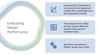
13. Evaluating
Model
Performance
R-squared (R2): Proportion of
the variance in the dependent
variable that is predictable from
the independent variable.
Mean Squared Error (MSE):
Average squared difference
between observed and
predicted values.
Root Mean Squared Error
(RMSE): Square root of MSE.

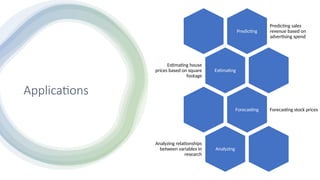
14. Applications
Predicting
Predicting sales
revenue based on
advertising spend
Estimating
Estimating house
prices based on square
footage
Forecasting Forecasting stock prices
Analyzing
Analyzing relationships
between variables in
research

15. Practice Example with
Code
• Import Libraries: Load necessary libraries.
• Load Dataset: Read the CSV file into a DataFrame.
• Define Model: Initialize the Linear Regression model.
• Prepare Data: Select features (X) and target (y).
• Split Data: Divide data into training and testing sets.
• Train Model: Fit the model to the training data.
• Make Predictions: Predict prices on the test set.
• Evaluate Model: Calculate Mean Squared Error (MSE)
and R² score.
• Link --
https://colab.research.google.com/drive/1uPdkArZtcg
CCFHIUzoB1-IysoLKzJ62B#scrollTo=1cldJVPwyzJm

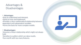
16. Advantages &
Disadvantages
• Advantages:
•Easy to understand and interpret.
•Quick to train and implement.
•Provides a clear mathematical relationship between
dependent and independent variables.
•Forms the basis for more complex models.
• Disadvantages:
•Assumes a linear relationship which might not always
hold.
•Sensitive to outliers which can skew results.
•Can overfit with too many features.

17. Conclusion
Predictive Modeling: Helps in predicting
outcomes based on input variables.
Understanding Relationships: Identifies
the strength and direction of
relationships between variables.
Versatility: Widely used in various fields
such as finance, real estate, and
research.
Foundation for Advanced Models:
Serves as the basis for more complex
statistical and machine learning models.

18. Bibliography
• https://www.ibm.com/topics/linear-regression
• https://www.geeksforgeeks.org/ml-linear-regression/
• https://www.statisticssolutions.com/free-resources/directory-of-statistical-analyses/what-
is-linear-regression/

19. Thank You