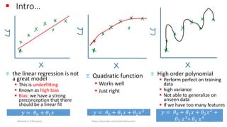
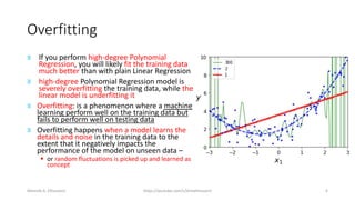
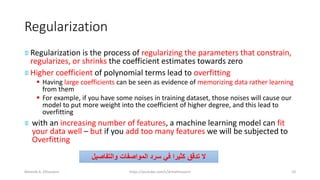
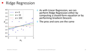
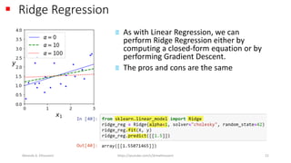
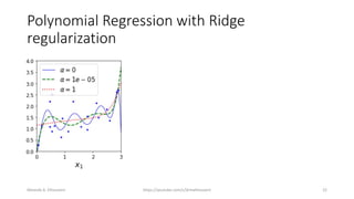
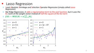
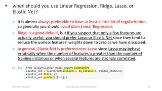
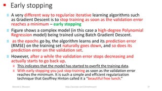
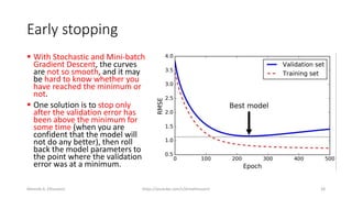
RegularizationDr. Mostafa A. Elhosseini
Ch. 4: Training Models
Dr. Mostafa A. Elhosseini
Mostafa A. Elhosseini https://youtube.com/c/drmelhosseini 2
Mostafa A. Elhosseini https://youtube.com/c/drmelhosseini 3
Agenda
≡ Regularization
Mostafa A. Elhosseini https://youtube.com/c/drmelhosseini 4
▪ Intro…
≡ the linear regression is not
a great model
▪ This is underfitting
▪ Known as high bias
▪ Bias: we have a strong
preconception that there
should be a linear fit
≡ Quadratic function
▪ Works well
▪ Just right
≡ High order polynomial
▪ Perform perfect on training
data
▪ high variance
▪ Not able to generalize on
unseen data
▪ If we have too many features
𝑦 = 𝜃0 + 𝜃1 𝑥 𝑦 = 𝜃0 + 𝜃1 𝑥 + 𝜃2 𝑥2 𝑦 = 𝜃0 + 𝜃1 𝑥 + 𝜃2 𝑥2 +
𝜃3 𝑥3
+ 𝜃4 𝑥4
Mostafa A. Elhosseini https://youtube.com/c/drmelhosseini 5
Overfitting
≡ If you perform high-degree Polynomial
Regression, you will likely fit the training data
much better than with plain Linear Regression
≡ high-degree Polynomial Regression model is
severely overfitting the training data, while the
linear model is underfitting it
≡ Overfitting: is a phenomenon where a machine
learning perform well on the training data but
fails to perform well on testing data
≡ Overfitting happens when a model learns the
details and noise in the training data to the
extent that it negatively impacts the
performance of the model on unseen data –
▪ or random fluctuations is picked up and learned as
concept
Mostafa A. Elhosseini https://youtube.com/c/drmelhosseini 6
Overfitting
≡ The model that will generalize best in this case is the quadratic
model.
▪ It makes sense since the data was generated using a quadratic model, but…
▪ In general you won’t know what function generated the data, so…
ꙮ How can you tell that your model is overfitting or underfitting the
data?
ꙮ how can you decide how complex your model should be?
Mostafa A. Elhosseini https://youtube.com/c/drmelhosseini 7
▪ How can you tell that your model is overfitting or
underfitting the data?
❶ Plotting hypothesis: is one way to decide – you may look for “curvy –
waggle”
▪ But does not always work
▪ Often have lots of features – harder to plot the data and visualize what feature to
keep and which one to throw out
❷ cross-validation metrics: If a model performs well on the training data
but generalizes poorly according to the cross-validation metrics, then
your model is overfitting.
▪ If it performs poorly on both, then it is underfitting.
❸ Learning curves: Another way is to look at the learning curves:
▪ these are plots of the model’s performance on the training set and the validation set
as a function of the training set size
▪ To generate the plots, simply train the model several times on different sized subsets
of the training set
Mostafa A. Elhosseini https://youtube.com/c/drmelhosseini 8
▪ Addressing overfitting
≡ If you have lots of features and little data – overfitting can be a problem
≡ simple way to regularize a polynomial model is to reduce the number of
polynomial degrees
≡ Reduce number of features:
▪ Manually select which features to keep
▪ Feature engineering – reduce numbers of features
▪ But, we lose information
▪ why do not we just stop adding features when we got an acceptable model!!!
▪ You do not know which features to drop, and even worse if it turns out that every
feature is fairly informative, which means that dropping some feature will likely ruin
the algorithm performance – the answer is regularization
≡ Regularization : keep all features, but reduce magnitude of parameters 𝜃
Mostafa A. Elhosseini https://youtube.com/c/drmelhosseini 9
Regularization
≡ Regularization is the process of regularizing the parameters that constrain,
regularizes, or shrinks the coefficient estimates towards zero
≡ Higher coefficient of polynomial terms lead to overfitting
▪ Having large coefficients can be seen as evidence of memorizing data rather learning
from them
▪ For example, if you have some noises in training dataset, those noises will cause our
model to put more weight into the coefficient of higher degree, and this lead to
overfitting
≡ with an increasing number of features, a machine learning model can fit
your data well – but if you add too many features we will be subjected to
Overfitting
‫والتفاصيل‬ ‫المواصفات‬ ‫سرد‬ ‫في‬ ‫كثيرا‬ ‫تدقق‬ ‫ال‬
Mostafa A. Elhosseini https://youtube.com/c/drmelhosseini 10
Recall: cost function
𝑱 =
𝟏
𝟐𝒎
෍
𝒊=𝟏
𝒎
𝒉 𝜽(𝑿 𝒊 ) − 𝒚(𝒊) 𝟐
≡ You parameter can be updated in any way, just to lower the MSE
value, and take care…
▪ The larger your parameters become, the higher the chance your model overfit
the data
Mostafa A. Elhosseini https://youtube.com/c/drmelhosseini 11
How to regularize?
• Penalize and make some of the 𝜃
parameters really small
• Like 𝜃3, 𝜃4
• 𝑱 =
𝟏
𝟐𝒎
σ𝒊=𝟏
𝒎
𝒉 𝜽(𝑿 𝒊 ) − 𝒚(𝒊) 𝟐
+ 𝟏𝟎𝟎𝟎 𝜽 𝟑
𝟐
+ 𝟏𝟎𝟎𝟎 𝜽 𝟒
𝟐
• The only way to minimize this function is to
make 𝜽 𝟑, 𝜽 𝟒 very small
• So here we end up with 𝜽 𝟑 and 𝜽 𝟒 being close
to zero
• Now we approximately have a quadratic
equation
• 𝑦 = 𝜃0 + 𝜃1 𝑥 + 𝜃2 𝑥2
𝑦 = 𝜃0 + 𝜃1 𝑥 + 𝜃2 𝑥2 +
𝜃3 𝑥3
+ 𝜃4 𝑥4
Mostafa A. Elhosseini https://youtube.com/c/drmelhosseini 12
How to regularize?
• Smaller values for parameters corresponds to a simpler hypothesis
• You get rid of some of the terms
• A simpler hypothesis is less prone to overfitting
• But, we do not know what are the high order terms
• How do we choose the ones to shrink?
• It is better to shrink all parameters
Mostafa A. Elhosseini https://youtube.com/c/drmelhosseini 13
▪ Main Goal
𝑱(𝜽) =
𝟏
𝟐𝒎
෍
𝒊=𝟏
𝒎
𝒉 𝜽(𝑿 𝒊
) − 𝒚(𝒊) 𝟐
+
𝝀
𝟐𝒎
෍
𝒋=𝟏
𝒏
𝜽𝑗
𝟐
≡ Minimize the cost function and restrict the parameters not to become too
large – thanks to the term of regularization
▪ 𝜆 is a constant the control the weight and importance of regularization term
▪ Control the trade off between the two goals
▪ Fit the training model very well
▪ Keep parameters small
▪ 𝑛 is the numbers of features
▪ By convention you do not penalize 𝜃0- minimization is from 𝜃1 onwards
▪ Minimizing the cost function consists of reducing MSE term and regularization term
≡ When parameter is updated to minimize MSE, and if it is becoming large, it will increase
the value of cost function by regularization term, and as a result it will be penalized and
updated to a small value
Mostafa A. Elhosseini https://youtube.com/c/drmelhosseini 14
Regularization
• If 𝜆 is very large we end up penalizing all the parameters, so all the
parameters end up being close to zero “Except 𝜃0”
• Like we get rid of all the terms – underfitting
• Too biased 𝒉 𝜽 = 𝜽 𝟎
• 𝜆 should be chosen carefully – not too big
Mostafa A. Elhosseini https://youtube.com/c/drmelhosseini 15
Regularization with Gradient Descent
• 𝑱(𝜽) =
𝟏
𝟐𝒎
σ𝒊=𝟏
𝒎
𝒉 𝜽(𝑿 𝒊 ) − 𝒚(𝒊) 𝟐
+ 𝝀 σ𝒋=𝟏
𝒏
𝜽𝑗
𝟐
• 𝜃0 is not regularized
• 𝜃0 = 𝜃0 −
𝛼
𝑚
σ𝑖=1
𝑚
ℎ 𝜃(𝑥 𝑖
) − 𝑦(𝑖)
𝑥0
(𝑖)
• 𝜃𝑗 = 𝜃𝑗 − 𝛼
1
𝑚
σ𝑖=1
𝑚
ℎ 𝜃(𝑥 𝑖 ) − 𝑦(𝑖) 𝑥𝑗
(𝑖) +
𝜆
𝑚
𝜃𝑗 𝑗 = 1,2,3, … , 𝑛
• 𝜃𝑗 = 𝜃𝑗 1 − 𝛼
𝜆
𝑚
−
𝛼
𝑚
σ𝑖=1
𝑚
ℎ 𝜃(𝑥 𝑖
) − 𝑦(𝑖)
𝑥𝑗
(𝑖)
𝑗 = 1,2,3, … , 𝑛
• The term 𝜃𝑗 1 − 𝛼
𝜆
𝑚
is going to be less than 1
• Usually learning rate is small and 𝑚 is large
• This term is often around 0.99 to 0.95
• i.e. shrink 𝜃𝑗 - the term on right is the same as before “Gradient descent
Mostafa A. Elhosseini https://youtube.com/c/drmelhosseini 16
Regularization
≡ For a linear model, regularization is typically achieved by
constraining the weights of the model.
≡ We will now look at Ridge Regression, Lasso Regression, and Elastic
Net, which implement three different ways to constrain the weights.
Mostafa A. Elhosseini https://youtube.com/c/drmelhosseini 17
Ridge Regression
≡ Also called Tikhonov regularization
≡ A regularization term equal to 𝝀 σ𝒋=𝟏
𝒏
𝜽𝑗
𝟐
is added to the cost function.
≡ Note that the regularization term should only be added to the cost function during
training
≡ Once the model is trained, you want to evaluate the model’s performance using the
unregularized performance measure
▪ It is quite common for the cost function used during training to be different from the performance
measure used for testing
▪ good training cost function should have optimization friendly derivatives, while the performance
measure used for testing should be as close as possible to the final objective
▪ A good example of this is a classifier trained using a cost function such as the log loss but
evaluated using precision/recall.
≡ It is important to scale the data (e.g., using a StandardScaler) before performing Ridge
Regression, as it is sensitive to the scale of the input features. This is true of most
regularized models.
Mostafa A. Elhosseini https://youtube.com/c/drmelhosseini 18
▪ Ridge Regression
≡ As with Linear Regression, we can
perform Ridge Regression either by
computing a closed-form equation or by
performing Gradient Descent.
≡ The pros and cons are the same
Mostafa A. Elhosseini https://youtube.com/c/drmelhosseini 19
▪ how to perform Ridge
Regression with Scikit-
Learn using a closed-
form solution
▪ using Stochastic Gradient Descent
▪ The penalty hyperparameter sets the type of regularization term to use.
▪ Specifying "l2" indicates that you want SGD to add a regularization term to
the cost function equal to half the square of the ℓ2 norm of the weight
vector:
▪ this is simply Ridge Regression.
Mostafa A. Elhosseini https://youtube.com/c/drmelhosseini 20
▪ Ridge Regression
≡ As with Linear Regression, we can
perform Ridge Regression either by
computing a closed-form equation or by
performing Gradient Descent.
≡ The pros and cons are the same
Mostafa A. Elhosseini https://youtube.com/c/drmelhosseini 21
Polynomial Regression with Ridge
regularization
Mostafa A. Elhosseini https://youtube.com/c/drmelhosseini 22
▪ Lasso Regression
≡ Least Absolute Shrinkage and Selection Operator Regression (simply called Lasso
Regression)
≡ like Ridge Regression, it adds a regularization term to the cost function, but it uses the
ℓ1 norm of the weight vector instead of half the square of the ℓ2 norm
≡ 𝑱 𝜽 = 𝑴𝑺𝑬 𝜽 + 𝜶 σ𝒊=𝟏
𝒏
𝜽𝒊
Mostafa A. Elhosseini https://youtube.com/c/drmelhosseini 23
Lasso Regression
≡ An important characteristic of Lasso Regression is that it tends to
completely eliminate the weights of the least important features
≡ Lasso Regression automatically performs feature selection and
outputs a sparse model (i.e., with few nonzero feature weights)
≡ Note that you could instead use an SGDRegressor(penalty="l1").
Mostafa A. Elhosseini https://youtube.com/c/drmelhosseini 24
Elastic Net
• Elastic Net is a middle ground between Ridge Regression and Lasso
Regression.
• The regularization term is a simple mix of both Ridge and Lasso’s
regularization terms, and you can control the mix ratio 𝑟.
• When 𝑟 = 0, Elastic Net is equivalent to Ridge Regression, and when
𝑟 = 1, it is equivalent to Lasso Regression
• 𝑱 𝜽 = 𝑴𝑺𝑬 𝜽 + 𝒓𝜶 σ𝒊=𝟏
𝒏
𝜽𝒊 +
𝟏−𝒓
𝟐
𝜶 σ𝒋=𝟏
𝒏
𝜽𝑖
𝟐
Mostafa A. Elhosseini https://youtube.com/c/drmelhosseini 25
▪ when should you use Linear Regression, Ridge, Lasso, or
Elastic Net?
≡ It is almost always preferable to have at least a little bit of regularization,
so generally you should avoid plain Linear Regression.
≡ Ridge is a good default, but if you suspect that only a few features are
actually useful, you should prefer Lasso or Elastic Net since they tend to
reduce the useless features’ weights down to zero as we have discussed.
≡ In general, Elastic Net is preferred over Lasso since Lasso may behave
erratically when the number of features is greater than the number of
training instances or when several features are strongly correlated.
Mostafa A. Elhosseini https://youtube.com/c/drmelhosseini 26
▪ Early stopping
≡ A very different way to regularize iterative learning algorithms such
as Gradient Descent is to stop training as soon as the validation error
reaches a minimum – early stopping
≡ Figure shows a complex model (in this case a high-degree Polynomial
Regression model) being trained using Batch Gradient Descent.
≡ as the epochs go by, the algorithm learns and its prediction error
(RMSE) on the training set naturally goes down, and so does its
prediction error on the validation set.
≡ However, after a while the validation error stops decreasing and
actually starts to go back up.
≡ This indicates that the model has started to overfit the training data.
≡ With early stopping you just stop training as soon as the validation error
reaches the minimum. It is such a simple and efficient regularization
technique that Geoffrey Hinton called it a “beautiful free lunch.”
Mostafa A. Elhosseini https://youtube.com/c/drmelhosseini 27
Early stopping
▪ With Stochastic and Mini-batch
Gradient Descent, the curves
are not so smooth, and it may
be hard to know whether you
have reached the minimum or
not.
▪ One solution is to stop only
after the validation error has
been above the minimum for
some time (when you are
confident that the model will
not do any better), then roll
back the model parameters to
the point where the validation
error was at a minimum.
Mostafa A. Elhosseini https://youtube.com/c/drmelhosseini 28

Lecture 19 chapter_4_regularized_linear_models

  • 1.
  • 2.
    Ch. 4: TrainingModels Dr. Mostafa A. Elhosseini Mostafa A. Elhosseini https://youtube.com/c/drmelhosseini 2
  • 3.
    Mostafa A. Elhosseinihttps://youtube.com/c/drmelhosseini 3
  • 4.
    Agenda ≡ Regularization Mostafa A.Elhosseini https://youtube.com/c/drmelhosseini 4
  • 5.
    ▪ Intro… ≡ thelinear regression is not a great model ▪ This is underfitting ▪ Known as high bias ▪ Bias: we have a strong preconception that there should be a linear fit ≡ Quadratic function ▪ Works well ▪ Just right ≡ High order polynomial ▪ Perform perfect on training data ▪ high variance ▪ Not able to generalize on unseen data ▪ If we have too many features 𝑦 = 𝜃0 + 𝜃1 𝑥 𝑦 = 𝜃0 + 𝜃1 𝑥 + 𝜃2 𝑥2 𝑦 = 𝜃0 + 𝜃1 𝑥 + 𝜃2 𝑥2 + 𝜃3 𝑥3 + 𝜃4 𝑥4 Mostafa A. Elhosseini https://youtube.com/c/drmelhosseini 5
  • 6.
    Overfitting ≡ If youperform high-degree Polynomial Regression, you will likely fit the training data much better than with plain Linear Regression ≡ high-degree Polynomial Regression model is severely overfitting the training data, while the linear model is underfitting it ≡ Overfitting: is a phenomenon where a machine learning perform well on the training data but fails to perform well on testing data ≡ Overfitting happens when a model learns the details and noise in the training data to the extent that it negatively impacts the performance of the model on unseen data – ▪ or random fluctuations is picked up and learned as concept Mostafa A. Elhosseini https://youtube.com/c/drmelhosseini 6
  • 7.
    Overfitting ≡ The modelthat will generalize best in this case is the quadratic model. ▪ It makes sense since the data was generated using a quadratic model, but… ▪ In general you won’t know what function generated the data, so… ꙮ How can you tell that your model is overfitting or underfitting the data? ꙮ how can you decide how complex your model should be? Mostafa A. Elhosseini https://youtube.com/c/drmelhosseini 7
  • 8.
    ▪ How canyou tell that your model is overfitting or underfitting the data? ❶ Plotting hypothesis: is one way to decide – you may look for “curvy – waggle” ▪ But does not always work ▪ Often have lots of features – harder to plot the data and visualize what feature to keep and which one to throw out ❷ cross-validation metrics: If a model performs well on the training data but generalizes poorly according to the cross-validation metrics, then your model is overfitting. ▪ If it performs poorly on both, then it is underfitting. ❸ Learning curves: Another way is to look at the learning curves: ▪ these are plots of the model’s performance on the training set and the validation set as a function of the training set size ▪ To generate the plots, simply train the model several times on different sized subsets of the training set Mostafa A. Elhosseini https://youtube.com/c/drmelhosseini 8
  • 9.
    ▪ Addressing overfitting ≡If you have lots of features and little data – overfitting can be a problem ≡ simple way to regularize a polynomial model is to reduce the number of polynomial degrees ≡ Reduce number of features: ▪ Manually select which features to keep ▪ Feature engineering – reduce numbers of features ▪ But, we lose information ▪ why do not we just stop adding features when we got an acceptable model!!! ▪ You do not know which features to drop, and even worse if it turns out that every feature is fairly informative, which means that dropping some feature will likely ruin the algorithm performance – the answer is regularization ≡ Regularization : keep all features, but reduce magnitude of parameters 𝜃 Mostafa A. Elhosseini https://youtube.com/c/drmelhosseini 9
  • 10.
    Regularization ≡ Regularization isthe process of regularizing the parameters that constrain, regularizes, or shrinks the coefficient estimates towards zero ≡ Higher coefficient of polynomial terms lead to overfitting ▪ Having large coefficients can be seen as evidence of memorizing data rather learning from them ▪ For example, if you have some noises in training dataset, those noises will cause our model to put more weight into the coefficient of higher degree, and this lead to overfitting ≡ with an increasing number of features, a machine learning model can fit your data well – but if you add too many features we will be subjected to Overfitting ‫والتفاصيل‬ ‫المواصفات‬ ‫سرد‬ ‫في‬ ‫كثيرا‬ ‫تدقق‬ ‫ال‬ Mostafa A. Elhosseini https://youtube.com/c/drmelhosseini 10
  • 11.
    Recall: cost function 𝑱= 𝟏 𝟐𝒎 ෍ 𝒊=𝟏 𝒎 𝒉 𝜽(𝑿 𝒊 ) − 𝒚(𝒊) 𝟐 ≡ You parameter can be updated in any way, just to lower the MSE value, and take care… ▪ The larger your parameters become, the higher the chance your model overfit the data Mostafa A. Elhosseini https://youtube.com/c/drmelhosseini 11
  • 12.
    How to regularize? •Penalize and make some of the 𝜃 parameters really small • Like 𝜃3, 𝜃4 • 𝑱 = 𝟏 𝟐𝒎 σ𝒊=𝟏 𝒎 𝒉 𝜽(𝑿 𝒊 ) − 𝒚(𝒊) 𝟐 + 𝟏𝟎𝟎𝟎 𝜽 𝟑 𝟐 + 𝟏𝟎𝟎𝟎 𝜽 𝟒 𝟐 • The only way to minimize this function is to make 𝜽 𝟑, 𝜽 𝟒 very small • So here we end up with 𝜽 𝟑 and 𝜽 𝟒 being close to zero • Now we approximately have a quadratic equation • 𝑦 = 𝜃0 + 𝜃1 𝑥 + 𝜃2 𝑥2 𝑦 = 𝜃0 + 𝜃1 𝑥 + 𝜃2 𝑥2 + 𝜃3 𝑥3 + 𝜃4 𝑥4 Mostafa A. Elhosseini https://youtube.com/c/drmelhosseini 12
  • 13.
    How to regularize? •Smaller values for parameters corresponds to a simpler hypothesis • You get rid of some of the terms • A simpler hypothesis is less prone to overfitting • But, we do not know what are the high order terms • How do we choose the ones to shrink? • It is better to shrink all parameters Mostafa A. Elhosseini https://youtube.com/c/drmelhosseini 13
  • 14.
    ▪ Main Goal 𝑱(𝜽)= 𝟏 𝟐𝒎 ෍ 𝒊=𝟏 𝒎 𝒉 𝜽(𝑿 𝒊 ) − 𝒚(𝒊) 𝟐 + 𝝀 𝟐𝒎 ෍ 𝒋=𝟏 𝒏 𝜽𝑗 𝟐 ≡ Minimize the cost function and restrict the parameters not to become too large – thanks to the term of regularization ▪ 𝜆 is a constant the control the weight and importance of regularization term ▪ Control the trade off between the two goals ▪ Fit the training model very well ▪ Keep parameters small ▪ 𝑛 is the numbers of features ▪ By convention you do not penalize 𝜃0- minimization is from 𝜃1 onwards ▪ Minimizing the cost function consists of reducing MSE term and regularization term ≡ When parameter is updated to minimize MSE, and if it is becoming large, it will increase the value of cost function by regularization term, and as a result it will be penalized and updated to a small value Mostafa A. Elhosseini https://youtube.com/c/drmelhosseini 14
  • 15.
    Regularization • If 𝜆is very large we end up penalizing all the parameters, so all the parameters end up being close to zero “Except 𝜃0” • Like we get rid of all the terms – underfitting • Too biased 𝒉 𝜽 = 𝜽 𝟎 • 𝜆 should be chosen carefully – not too big Mostafa A. Elhosseini https://youtube.com/c/drmelhosseini 15
  • 16.
    Regularization with GradientDescent • 𝑱(𝜽) = 𝟏 𝟐𝒎 σ𝒊=𝟏 𝒎 𝒉 𝜽(𝑿 𝒊 ) − 𝒚(𝒊) 𝟐 + 𝝀 σ𝒋=𝟏 𝒏 𝜽𝑗 𝟐 • 𝜃0 is not regularized • 𝜃0 = 𝜃0 − 𝛼 𝑚 σ𝑖=1 𝑚 ℎ 𝜃(𝑥 𝑖 ) − 𝑦(𝑖) 𝑥0 (𝑖) • 𝜃𝑗 = 𝜃𝑗 − 𝛼 1 𝑚 σ𝑖=1 𝑚 ℎ 𝜃(𝑥 𝑖 ) − 𝑦(𝑖) 𝑥𝑗 (𝑖) + 𝜆 𝑚 𝜃𝑗 𝑗 = 1,2,3, … , 𝑛 • 𝜃𝑗 = 𝜃𝑗 1 − 𝛼 𝜆 𝑚 − 𝛼 𝑚 σ𝑖=1 𝑚 ℎ 𝜃(𝑥 𝑖 ) − 𝑦(𝑖) 𝑥𝑗 (𝑖) 𝑗 = 1,2,3, … , 𝑛 • The term 𝜃𝑗 1 − 𝛼 𝜆 𝑚 is going to be less than 1 • Usually learning rate is small and 𝑚 is large • This term is often around 0.99 to 0.95 • i.e. shrink 𝜃𝑗 - the term on right is the same as before “Gradient descent Mostafa A. Elhosseini https://youtube.com/c/drmelhosseini 16
  • 17.
    Regularization ≡ For alinear model, regularization is typically achieved by constraining the weights of the model. ≡ We will now look at Ridge Regression, Lasso Regression, and Elastic Net, which implement three different ways to constrain the weights. Mostafa A. Elhosseini https://youtube.com/c/drmelhosseini 17
  • 18.
    Ridge Regression ≡ Alsocalled Tikhonov regularization ≡ A regularization term equal to 𝝀 σ𝒋=𝟏 𝒏 𝜽𝑗 𝟐 is added to the cost function. ≡ Note that the regularization term should only be added to the cost function during training ≡ Once the model is trained, you want to evaluate the model’s performance using the unregularized performance measure ▪ It is quite common for the cost function used during training to be different from the performance measure used for testing ▪ good training cost function should have optimization friendly derivatives, while the performance measure used for testing should be as close as possible to the final objective ▪ A good example of this is a classifier trained using a cost function such as the log loss but evaluated using precision/recall. ≡ It is important to scale the data (e.g., using a StandardScaler) before performing Ridge Regression, as it is sensitive to the scale of the input features. This is true of most regularized models. Mostafa A. Elhosseini https://youtube.com/c/drmelhosseini 18
  • 19.
    ▪ Ridge Regression ≡As with Linear Regression, we can perform Ridge Regression either by computing a closed-form equation or by performing Gradient Descent. ≡ The pros and cons are the same Mostafa A. Elhosseini https://youtube.com/c/drmelhosseini 19
  • 20.
    ▪ how toperform Ridge Regression with Scikit- Learn using a closed- form solution ▪ using Stochastic Gradient Descent ▪ The penalty hyperparameter sets the type of regularization term to use. ▪ Specifying "l2" indicates that you want SGD to add a regularization term to the cost function equal to half the square of the ℓ2 norm of the weight vector: ▪ this is simply Ridge Regression. Mostafa A. Elhosseini https://youtube.com/c/drmelhosseini 20
  • 21.
    ▪ Ridge Regression ≡As with Linear Regression, we can perform Ridge Regression either by computing a closed-form equation or by performing Gradient Descent. ≡ The pros and cons are the same Mostafa A. Elhosseini https://youtube.com/c/drmelhosseini 21
  • 22.
    Polynomial Regression withRidge regularization Mostafa A. Elhosseini https://youtube.com/c/drmelhosseini 22
  • 23.
    ▪ Lasso Regression ≡Least Absolute Shrinkage and Selection Operator Regression (simply called Lasso Regression) ≡ like Ridge Regression, it adds a regularization term to the cost function, but it uses the ℓ1 norm of the weight vector instead of half the square of the ℓ2 norm ≡ 𝑱 𝜽 = 𝑴𝑺𝑬 𝜽 + 𝜶 σ𝒊=𝟏 𝒏 𝜽𝒊 Mostafa A. Elhosseini https://youtube.com/c/drmelhosseini 23
  • 24.
    Lasso Regression ≡ Animportant characteristic of Lasso Regression is that it tends to completely eliminate the weights of the least important features ≡ Lasso Regression automatically performs feature selection and outputs a sparse model (i.e., with few nonzero feature weights) ≡ Note that you could instead use an SGDRegressor(penalty="l1"). Mostafa A. Elhosseini https://youtube.com/c/drmelhosseini 24
  • 25.
    Elastic Net • ElasticNet is a middle ground between Ridge Regression and Lasso Regression. • The regularization term is a simple mix of both Ridge and Lasso’s regularization terms, and you can control the mix ratio 𝑟. • When 𝑟 = 0, Elastic Net is equivalent to Ridge Regression, and when 𝑟 = 1, it is equivalent to Lasso Regression • 𝑱 𝜽 = 𝑴𝑺𝑬 𝜽 + 𝒓𝜶 σ𝒊=𝟏 𝒏 𝜽𝒊 + 𝟏−𝒓 𝟐 𝜶 σ𝒋=𝟏 𝒏 𝜽𝑖 𝟐 Mostafa A. Elhosseini https://youtube.com/c/drmelhosseini 25
  • 26.
    ▪ when shouldyou use Linear Regression, Ridge, Lasso, or Elastic Net? ≡ It is almost always preferable to have at least a little bit of regularization, so generally you should avoid plain Linear Regression. ≡ Ridge is a good default, but if you suspect that only a few features are actually useful, you should prefer Lasso or Elastic Net since they tend to reduce the useless features’ weights down to zero as we have discussed. ≡ In general, Elastic Net is preferred over Lasso since Lasso may behave erratically when the number of features is greater than the number of training instances or when several features are strongly correlated. Mostafa A. Elhosseini https://youtube.com/c/drmelhosseini 26
  • 27.
    ▪ Early stopping ≡A very different way to regularize iterative learning algorithms such as Gradient Descent is to stop training as soon as the validation error reaches a minimum – early stopping ≡ Figure shows a complex model (in this case a high-degree Polynomial Regression model) being trained using Batch Gradient Descent. ≡ as the epochs go by, the algorithm learns and its prediction error (RMSE) on the training set naturally goes down, and so does its prediction error on the validation set. ≡ However, after a while the validation error stops decreasing and actually starts to go back up. ≡ This indicates that the model has started to overfit the training data. ≡ With early stopping you just stop training as soon as the validation error reaches the minimum. It is such a simple and efficient regularization technique that Geoffrey Hinton called it a “beautiful free lunch.” Mostafa A. Elhosseini https://youtube.com/c/drmelhosseini 27
  • 28.
    Early stopping ▪ WithStochastic and Mini-batch Gradient Descent, the curves are not so smooth, and it may be hard to know whether you have reached the minimum or not. ▪ One solution is to stop only after the validation error has been above the minimum for some time (when you are confident that the model will not do any better), then roll back the model parameters to the point where the validation error was at a minimum. Mostafa A. Elhosseini https://youtube.com/c/drmelhosseini 28