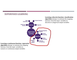
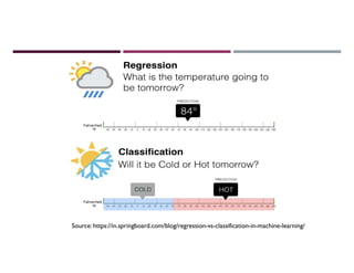
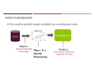
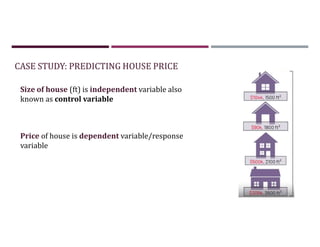
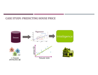
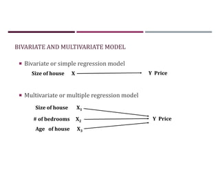
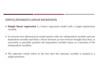
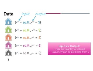
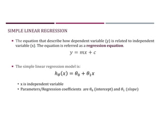
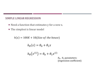
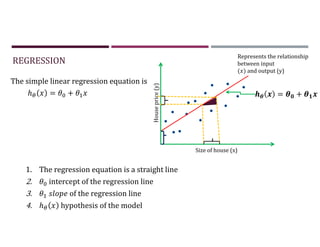
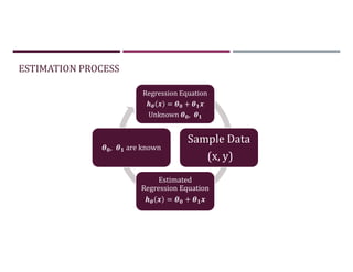
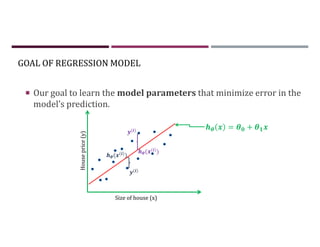
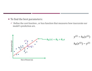
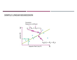
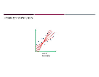
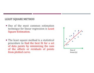
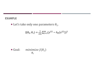
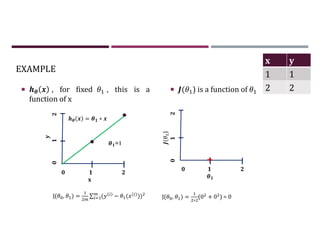
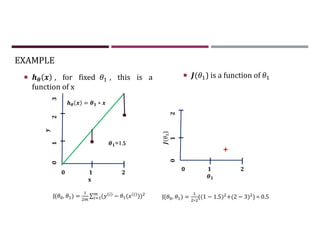
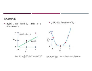
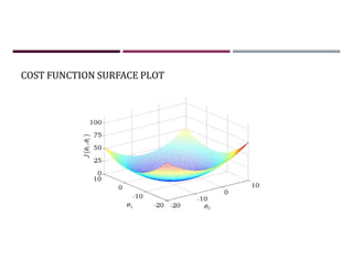
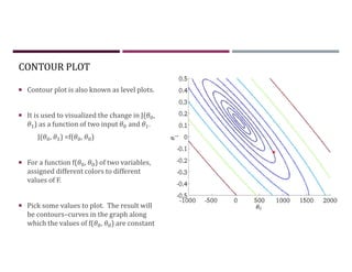
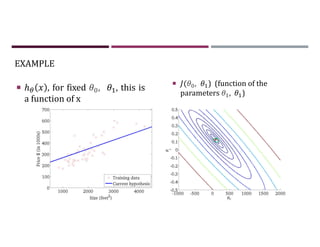
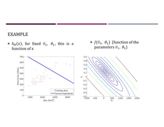
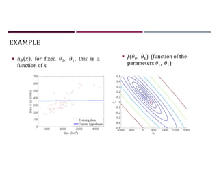
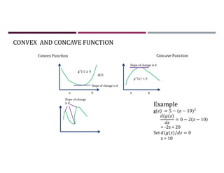
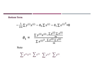
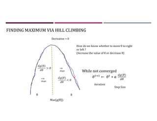
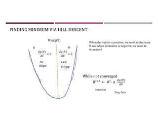
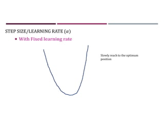
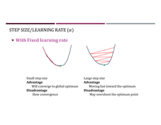
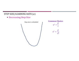
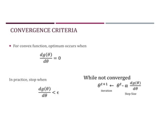
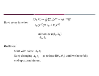
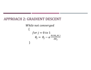
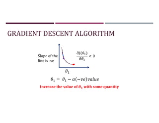
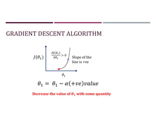
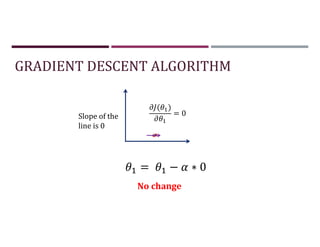
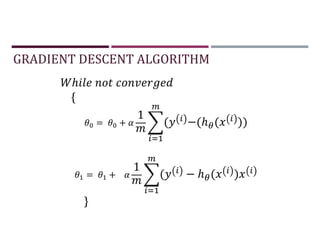
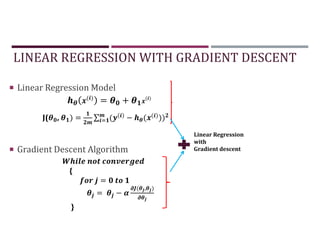
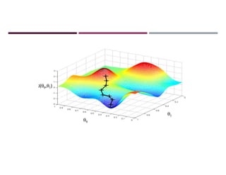
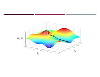
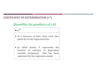
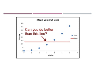
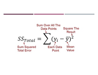
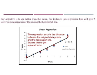
This document discusses supervised learning and regression analysis in machine learning. It defines regression as a technique used to predict continuous target variables by identifying relationships between input features and output variables. Simple linear regression fits a linear function to the data to predict a dependent, or target, variable from an independent variable. Gradient descent is introduced as an optimization algorithm that can be used to fit simple linear regression models by minimizing a cost function.

1. Supervised Learning
Regression
Assistant Professor, Department of Computer Science & Engineering
PDPM-Indian Institute of Information Technology Design and
Manufacturing, Jabalpur
Dumna Airport Road - 482005
Email: kusum@iiitdmj.ac.in
Dr. Kusum Kumari Bharti

2. AGENDA
Outlines
Supervised Learning
Regression
Case Study
Simple Linear Regression
Summary

3. RECAP
Source: https://blog.digitalogy.co/the-difference-between-artificial-intelligence-machine-learning-and-deep-learning/
RECAP

4. SUPERVISED LEARNING
Image Source: https://www.javatpoint.com/supervised-machine-learning

5. SUPERVISED LEARNING
Learning a discrete function- classification
algorithm attempt to estimate the mapping
function from the input variables to
discrete or categorical output variables
Learning a continuous function- regression
algorithm attempt to estimate the mapping
function from the input variables to
numeric or continuous output variables
SUPERVISED LEARNING

6. CLASSIFICATION VS REGRESSION
Classification Regression

7. Source: https://in.springboard.com/blog/regression-vs-classification-in-machine-learning/

8. REGRESSION ANALYSIS

9. WHAT IS REGRESSION
 It is used to predict target variables on a continuous scale.
WHAT IS REGRESSION
Map x  y
Identify
Relationship
Dataset
Regression

10. How much will your salary be ?
Depends on x = performance in course, quality of projects, etc….
SALARY AFTER COMPLETING THE COURSE

11. STOCK PREDICTION
 Predict the price of the stock (y)
 Depends on x
 Recent history of stock price
 News events
 Related commodities
STOCK PREDICTION

12.  How many people will retweet your tweet? (y)
 Depends on x = # followers, # of followers of followers, features of text tweeted,
popularity of hashtag, # of past retweets…….
TWEET POPULARITY

13. REGRESSION
 Other application
 How many customers will arrive at our website next week?
 How many tv’s will sell next week?
 Predicting the sales of a company in future months.
 Can we predict someone’s income from their click through information's?

14. REGRESSION ANALYSIS
 Regression Analysis is a statistical tool for investigating the
relationship between a dependent variable and one or more
independent variables/explanatory variable.
 Regression analysis is widely used for prediction and
forecasting

15. INDEPENDENT AND DEPENDENT VARIABLE
 Independent Variable (Explanatory Variable):
A variable whose value does not change by the effect of other variables and
is used to manipulate the dependent variable/target variable. It is often denoted
by X
 Dependent Variable
A variable whose value changes when there is any manipulation in the
values of independent variable. It is often denoted by Y

16. CASE STUDY: PREDICTING HOUSE PRICE

17. CASE STUDY: PREDICTING HOUSE PRICE
Size of house (ft) is independent variable also
known as control variable
Price of house is dependent variable/response
variable

18. WHAT IS REGRESSION
CASE STUDY: PREDICTING HOUSE PRICE
Dataset
Regression

19. BIVARIATE AND MULTIVARIATE MODEL
 Bivariate or simple regression model
 Multivariate or multiple regression model
Size of house X Y Price
Age of house X3
# of bedrooms X2
Size of house X1
Y Price

20. SIMPLE/BIVARIATE LINEAR REGRESSION
 Simple linear regression is a linear regression model with a single explanatory
variable.
 It concerns two-dimensional sample points with one independent variable and one
dependent variable and finds a linear function (a non-vertical straight line) that, as
accurately as possible, predicts the dependent variable values as a function of the
independent variables.
 The adjective simple refers to the fact that the outcome variable is related to a
single predictor.

21. HOW MUCH IS MY HOUSE WORTH?

22. LOOK AT RECENT SALES IN MY NEIGHBORHOOD
 How much did they sell for ?

23. ( )
( )
( )
( )
( )
( )
( )
( )
( )
( )

24. REGRESSION (HOUSE PRICE PREDICTION)
Size of house (ft) is independent
variable also known as control
variable
Price of house is dependent
Variable/response variable
Scatter plot is a mathematical diagram to
display values of two variables for a set of data.
Dependent
Variable Independent Variable
Scatter plots are used to investigates the position
relationship between the variables
,

25. SIMPLE LINEAR REGRESSION
We want to fit the best line (linear function
Y = f(X)) to explain the data
House Price Predication

26. SIMPLE LINEAR REGRESSION

27. SIMPLE LINEAR REGRESSION
 The equation that describe how dependent variable (y) is related to independent
variable (x). The equation is referred as a regression equation.
= +
 The simple linear regression model is:
• x is independent variable
• Parameters/Regression coefficients are (intercept) and ( )
ℎ = +

28. SIMPLE LINEAR REGRESSION
 Need a function that estimates y for a new x.
 The simplest is linear model
ℎ = 100 + 10( ℎ ℎ )
ℎ = +
ℎ ( )
= + ( )
, parameters:
(regression coefficient)

29. REGRESSION
Represents the relationship
between input
( ) and output (y)
House
price
(y)
= +
Size of house (x)
1. The regression equation is a straight line
2. intercept of the regression line
3. of the regression line
4. ℎ hypothesis of the model
ℎ = +
The simple linear regression equation is

30. ESTIMATION PROCESS
Regression Equation
= +
Unknown ,
Sample Data
(x, y)
Estimated
Regression Equation
= +
, are known

31. GOAL OF REGRESSION MODEL
 Our goal to learn the model parameters that minimize error in the
model’s prediction.
Size of house (x)
House
price
(y)
= +
( ( ))
( )
( ( ))
( )

32.  To find the best parameters:
 Define the cost function , or loss function that measures how inaccurate our
model’s prediction are.
Size of house (x)
House
price
(y)
= +
( ( ))
( )
( ( ))
( )
( )
− ℎ ( ( )
)
ℎ ( ( )
) − ( )

33. SIMPLE LINEAR REGRESSION
Hθ(x) =
j
Parameter :
Regression coefficient

34. EFFECTS OF PARAMETERS ON LINE PLACEMENT
= . + ∗
= + . ∗
= + . ∗
0 1 2 3
0
1
2
3
x y
1 1
2 2
3 3

35. EFFECTS OF PARAMETERS ON LINE PLACEMENT
Example
Suppose x = 2.5
ℎ = 1 + 0.5 ∗
Predict the outcome
ℎ =1 + 0.5 *2.5
= 2.25
x y
1 1
2 2
3 3
= . + ∗
= + . ∗
= + . ∗
0 1 2 3
0
1
2
3

36. ESTIMATION PROCESS
Size of
house (x)

37. LEAST SQUARE METHOD
 One of the most common estimation
technique for linear regression is Least
Square Estimation.
 The least square method is a statistical
procedure to find the best fit for a set
of data points by minimizing the sum
of the offsets or residuals of points
from plotted curve.
Size of
house (x)

38. Least Square Method
is residual error (RSS) in the ith observation
= + ( )
+
= − ℎ ( )
J( , ) = ( − ℎ ( ( )
)) +( − ℎ ( ( )
)) +( − ℎ ( ( )
))
+ ⋯ … … … … . +
ℎ

39. So, our aim to minimize the total error.
J( , ) = ∑ ( − ℎ ( ( )
))
,
J( , )
Cost Function

40. EXAMPLE
 Let’s take only one parameters .
 Goal: ( )
J( , ) = ∑ ( − ℎ ( ( )
))

41. EXAMPLE
 , for fixed , this is a
function of x
 ( ) is a function of
= ∗
0 1 2
x
y
0
1
2
0 1 2
(
)
0
1
2
J( , ) = ∑ ( − ( ( ))) J( , ) =
∗
(0 + 0 ) = 0
=1
x y
1 1
2 2

42. EXAMPLE
 , for fixed , this is a
function of x
 ( ) is a function of
= ∗
0 1 2
x
y
0
1
2
3
0 1 2
(
)
0
1
2
J( , ) = ∑ ( − ( ( ))) J( , ) =
∗
((1 − 1.5) +(2 − 3) ) = 0.5
=1.5

43. EXAMPLE
 , for fixed , this is a
function of x
 ( ) is a function of
= ∗
0 1 2
x
y
0
1
2
0 1 2
(
)
0
1
2
J( , ) = ∑ ( − ( ( ))) J( , ) =
∗
((1 − 0.75) +(2 − 1.5) ) = 0.07
=.75

44. COST FUNCTION SURFACE PLOT

45. CONTOUR PLOT
 Contour plot is also known as level plots.
 It is used to visualized the change in J( ,
) as a function of two input and .
J( , ) =f( , )
 For a function f( , ) of two variables,
assigned different colors to different
values of F.
 Pick some values to plot. The result will
be contours–curves in the graph along
which the values of f( , ) are constant

46. EXAMPLE
 ℎ , for fixed , , this is
a function of x
 ( , ) (function of the
parameters , )

47. EXAMPLE
 ℎ , for fixed , , this is a
function of x
 ( , ) (function of the
parameters , )

48. EXAMPLE
 ℎ , for fixed , , this is a
function of x
 ( , ) (function of the
parameters , )

49. SUMMARY
Hypothesis
Parameters
Cost Function
Goal
ℎ = +
,
J( , ) = ∑ ( − ℎ ( ( )
))
( , )
,

50. CONVEX AND CONCAVE FUNCTION
g(z)
b
a
a b
Slope of change is 0
Slope of change is 0
Slope of change
is 0
g′′( ) ≥ 0
< 0
Example
g( ) = 5 − ( − 10)
( ( )
= 0 − 2 − 10
= -2z + 20
Set ( ( )⁄ = 0
z = 10
Concave Function
Convex Function

51. COMPUTE THE GRADIENT
J( , ) = ∑ ( − ℎ ( ( )
))
ℎ ( ) = + ( )

52. ( , ) =
1
2
( − ( + ( )
))
J( , )
=
1
2
( − ( + ( )
))
J( , )
=
1
2
( − ( + ( )
))

53. J( , )
=
1
2
( − ℎ ( ( )
))
=
1
( −( + ))(−1)
J( , )
=
1
2
( − ( + ( )
))
=
1
( − ( + ( )
)) . (− ( )
)

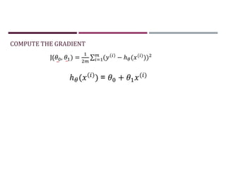
54. COMPUTE THE GRADIENT
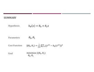
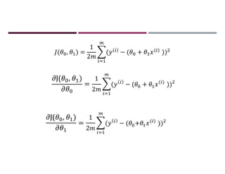
Putting it together
J( , ) = ∑ ( − ℎ ( ( )
))
J( , ) =
∑ [ ( )]
∑ [ ( ( ) )] . ( ( ))

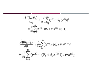
55. APPROACH 1 : SET GRADIENT = 0
J( , ) =
∑ [ ( )]
∑ [ ( ( ) )] . ( ( ))
Top Term
=
∑
−
∑

56. Bottom Term
− ∑ − ∑ − ∑ =0
=
∑
∑ ∑
∑
∑ ∑
Note

57. FINDING MAXIMUM VIA HILL CLIMBING
Max(g(θ))
+ve
slope
-ve
slope
How do we know whether to move θ to right
or left ?
(Increase the value of θ or decrease θ)
θ θ
( )
< 0
( )
> 0
While not converged
← + α
( )
iteration
Step Size
Derivative = 0

58. FINDING MINIMUM VIA HILL DESCENT
Min(g(θ)
+ve
slope
-ve
slope
( )
> 0
( )
< 0
θ θ
While not converged
← - α
( )
iteration
Step Size
When derivative is positive, we want to decrease
and when derivative is negative, we want to
increase

59. STEP SIZE/LEARNING RATE ( )
 With Fixed learning rate
Slowly reach to the optimum
position

60. STEP SIZE/LEARNING RATE ( )
 With Fixed learning rate
Small step size
Advantage
Will converge to global optimum
Disadvantage
Slow convergence
Large step size
Advantage
Moving fast toward the optimum
Disadvantage
May overshoot the optimum point

61. STEP SIZE/LEARNING RATE ( )
 Decreasing Step Size
Common Choice:
α =
α =
Step size is scheduled

62. CONVERGENCE CRITERIA
 For convex function, optimum occurs when
In practice, stop when
= 0
While not converged
← - α
( )
iteration
Step Size
< ϵ

63. GRADIENT DESCENT
Gradient descent is an optimization algorithm used to find the values of parameters
(coefficients) of a function (f) that minimizes a cost function (cost).

64. Have some function
Outlines:
Start with some
Keep changing to reduce J( , ) until we hopefully
end up at a minimum.
( , )
,
,
J( , ) = ∑ ( − ℎ ( ( )))
ℎ ( )= + ( )
,

65. APPROACH 2: GRADIENT DESCENT
ℎ
{
= 0 1
= −
( , )
}

66. GRADIENT DESCENT ALGORITHM
Slope of the
line is -ve
( )
< 0
= − −
Increase the value of with some quantity

67. GRADIENT DESCENT ALGORITHM
Slope of the
line is +ve
( )
> 0
= − +
( )
Decrease the value of with some quantity

68. GRADIENT DESCENT ALGORITHM
Slope of the
line is 0
( )
= 0
= − ∗ 0
No change

69. GRADIENT DESCENT ALGORITHM
ℎ
{
= +
1
( −(ℎ ( ))
= +
1
( − ℎ ( )
}

70. LINEAR REGRESSION WITH GRADIENT DESCENT
 Linear Regression Model
 Gradient Descent Algorithm
( )
= + ( )
J( , ) = ∑ ( − ( ( )))
{
=
= −
( , )
}
Linear Regression
with
Gradient descent

73. GRADIENT DESCENT ALGORITHM
 Types of Gradient Descent Algorithm
 Stochastic gradient descent
 SGD randomly picks one data point from the whole data set at each iteration.
 Batch gradient descent
 Every step of gradient descent uses all the training examples
 Mini-batch gradient descent
 A balance between the goodness of gradient descent and speed of SGD.
 sample a small number of data points instead of just one point at each step.

74. COEFFICIENT OF DETERMINATION ( )

 Is a measure of how close each data
point fits to the regression line.
 In other words, it represents the
fraction of variance in dependent
variable (response) that has been
explained by the regression model
Quantifies the goodness of a fit.

76.  R-Squared is a way of measuring how much better than the mean line
you have done based on summed squared error.

79. Our objective is to do better than the mean. For instance this regression line will give A
lower sum squared error than using the horizontal line.

81. Ideally, you would have zero regression error, i.e. Your regression line would perfectly
match the data. In that case you would get an r-squared value of 1

82. EXAMPLE
Source: http://www.fairlynerdy.com/what-is-r-squared/
Regression Line
X Y SS_Total Y = 6x -5
SS_Regression
0 0 169 -5 5 25
1 1 144 1 0 0
2 4 81 7 -3 9
3 9 16 13 -4 16
4 16 9 19 -3 9
5 25 144 25 0 0
6 36 529 31 5 25
Average 13
Total 1092 84
R-squared
0.923

83. LINEAR REGRESSION WITH MULTIPLE VARIABLES
POLYNOMIAL REGRESSION

84. INCORPORATING COMPLEX INFORMATION
R Squared:
0.18231625879420676
R Squared:
0.9432150416451027

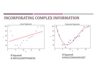
85. INCORPORATING COMPLEX INFORMATION
Intercept: 49.67777777777776
Coefficient: [5.01666667]
R Squared: 0.9757431074095347
Intercept: 7.27106067219556
Coefficient: [7.25447403]
R Squared: 0.9503677766997879

86. MORE COMPLEX FUNCTION OF SINGLE INPUT
Intercept: 7.27106067219556
Coefficient: [7.25447403]
R Squared: 0.9503677766997879
Slope: [0. 4.3072556 0.24072435]
Intercept: 13.026878767297461
R Squared: 0.9608726568678714