Supervised Learning (Part2)
Md. Shahidul Islam
Assistant Professor
Dept. of CSE, University of Asia Pacific
2.
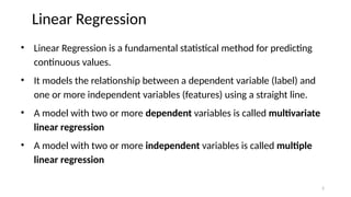
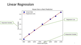
Linear Regression
• LinearRegression is a fundamental statistical method for predicting
continuous values.
• It models the relationship between a dependent variable (label) and
one or more independent variables (features) using a straight line.
• A model with two or more dependent variables is called multivariate
linear regression
• A model with two or more independent variables is called multiple
linear regression
2
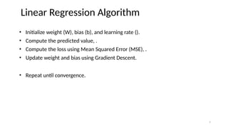
• Initialize weight(W), bias (b), and learning rate ().
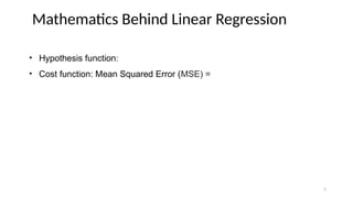
• Compute the predicted value, .
• Compute the loss using Mean Squared Error (MSE), .
• Update weight and bias using Gradient Descent.
• Repeat until convergence.
Linear Regression Algorithm
7
8.
• Real worldapplications have multiple independent variables
• Multiple linear regression comes into action
• The formulation is similar to the simple linear regression
• Gradient Descent for Multiple Linear Regression
Multiple Linear Regression
8
9.
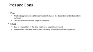
• Pros
• Simplemodel
• Computationally efficient
• Interpretability of the Output
• Cons
• Overly-Simplistic
• Linearity Assumption
• Severely affected by Outliers
Pros and Cons
9
10.
• Describes therelationship between the independent variable x and the
dependent variable y using an nth
-degree polynomial in x
• Characterizes fitting a nonlinear relationship between the x value and the
conditional mean of y
• Types
• Linear – if degree as 1
• Quadratic – if degree as 2
• Cubic – if degree as 3 and goes on, on the basis of degree.
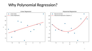
Polynomial Regression
10
• Pros
• Thebest approximation of the connection between the dependent and independent
variables
• Can accommodate a wide range of functions
• Cons
• One or two outliers in the data might have a significant impact
• Fewer model validation methods for detecting outliers in nonlinear regression
Pros and Cons
12
13.
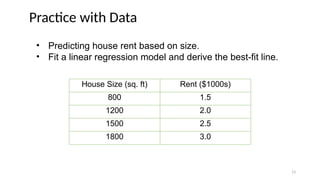
Practice with Data
HouseSize (sq. ft) Rent ($1000s)
800 1.5
1200 2.0
1500 2.5
1800 3.0
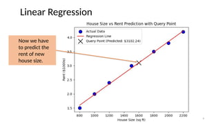
• Predicting house rent based on size.
• Fit a linear regression model and derive the best-fit line.
13
#3 import numpy as np
import matplotlib.pyplot as plt
# Sample data: House size (sq ft) and Rent (in $1000s)
data = {
"House Size": [800, 1000, 1200, 1500, 1800, 2000, 2200],
"Rent": [1.5, 2.0, 2.4, 3.0, 3.5, 3.8, 4.2]
}
# Fit a simple linear regression model
house_size = np.array(data["House Size"]).reshape(-1, 1)
rent = np.array(data["Rent"])
# Perform linear regression
from sklearn.linear_model import LinearRegression
model = LinearRegression()
model.fit(house_size, rent)
predicted_rent = model.predict(house_size)
# Scatter plot
plt.scatter(data["House Size"], data["Rent"], color='blue', label="Actual Data", edgecolors='k', s=100)
plt.plot(data["House Size"], predicted_rent, color='red', label="Regression Line")
# Labels and title
plt.xlabel("House Size (sq ft)")
plt.ylabel("Rent ($1000s)")
plt.title("House Size vs Rent Prediction")
plt.legend()
# Display plot
plt.show()
#4 import numpy as np
import matplotlib.pyplot as plt
from sklearn.linear_model import LinearRegression
# Sample data: House size (sq ft) and Rent (in $1000s)
data = {
"House Size": [800, 1000, 1200, 1500, 1800, 2000, 2200],
"Rent": [1.5, 2.0, 2.4, 3.0, 3.5, 3.8, 4.2]
}
# Convert data into numpy arrays
house_size = np.array(data["House Size"]).reshape(-1, 1)
rent = np.array(data["Rent"])
# Initialize and train the Linear Regression model
model = LinearRegression()
model.fit(house_size, rent)
# Predict rent for a new house size (query point)
query_house_size = np.array([[1600]]) # House size: 1600 sq ft
predicted_rent = model.predict(query_house_size)[0]
# Scatter plot of actual data
plt.scatter(data["House Size"], data["Rent"], color='blue', label="Actual Data", edgecolors='k', s=100)
# Regression line
predicted_rent_line = model.predict(house_size)
plt.plot(data["House Size"], predicted_rent_line, color='red', label="Regression Line")
# Mark the query point
plt.scatter(query_house_size, predicted_rent, color='black', marker='x', s=200, label=f'Query Point (Predicted: ${predicted_rent*1000:.2f})')
# Labels and title
plt.xlabel("House Size (sq ft)")
plt.ylabel("Rent ($1000s)")
plt.title("House Size vs Rent Prediction with Query Point")
plt.legend()
# Display plot
plt.show()
#6 import numpy as np
import matplotlib.pyplot as plt
from sklearn.linear_model import LinearRegression
# Dataset: House size vs Rent with some variations
data = {
"House Size": [800, 1000, 1200, 1500, 1800, 2000, 2200],
"Rent": [1.2, 2.5, 2.0, 3.5, 3.2, 4.5, 4.0] # Slightly scattered values
}
# Convert data into numpy arrays
house_size = np.array(data["House Size"]).reshape(-1, 1)
rent = np.array(data["Rent"])
# Create 3 different regression models
model1 = LinearRegression()
model2 = LinearRegression()
model3 = LinearRegression()
# Different training data for variety
house_size1, rent1 = house_size[:-1], rent[:-1] # Exclude last point
house_size2, rent2 = house_size[1:], rent[1:] # Exclude first point
house_size3, rent3 = house_size, rent # Full dataset
# Fit models
model1.fit(house_size1, rent1)
model2.fit(house_size2, rent2)
model3.fit(house_size3, rent3)
# Predictions
pred_rent1 = model1.predict(house_size)
pred_rent2 = model2.predict(house_size)
pred_rent3 = model3.predict(house_size)
# Compute MSE
mse1 = np.mean((rent - pred_rent1) ** 2)
mse2 = np.mean((rent - pred_rent2) ** 2)
mse3 = np.mean((rent - pred_rent3) ** 2)
# Scatter plot for actual data
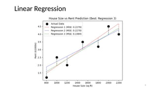
plt.scatter(data["House Size"], data["Rent"], color='black', label="Actual Data", edgecolors='k', s=100)
# Regression lines (all dotted)
plt.plot(data["House Size"], pred_rent1, color='red', linestyle="dotted", label=f"Regression 1 (MSE: {mse1:.4f})")
plt.plot(data["House Size"], pred_rent2, color='blue', linestyle="dotted", label=f"Regression 2 (MSE: {mse2:.4f})")
plt.plot(data["House Size"], pred_rent3, color='green', linestyle="dotted", label=f"Regression 3 (MSE: {mse3:.4f})")
# Draw vertical error lines to the data points
for i in range(len(data["House Size"])):
plt.plot([data["House Size"][i], data["House Size"][i]], [rent[i], pred_rent1[i]], 'r--', alpha=0.5) # Regression 1 error lines
plt.plot([data["House Size"][i], data["House Size"][i]], [rent[i], pred_rent2[i]], 'b--', alpha=0.5) # Regression 2 error lines
plt.plot([data["House Size"][i], data["House Size"][i]], [rent[i], pred_rent3[i]], 'g--', alpha=0.5) # Regression 3 error lines
# Choose the best model based on MSE
best_model = min((mse1, "Regression 1"), (mse2, "Regression 2"), (mse3, "Regression 3"))
plt.title(f"House Size vs Rent Prediction (Best: {best_model[1]})")
# Labels
plt.xlabel("House Size (sq ft)")
plt.ylabel("Rent ($1000s)")
plt.legend()
# Display plot
plt.show()
#11 import numpy as np
import matplotlib.pyplot as plt
from sklearn.linear_model import LinearRegression
from sklearn.preprocessing import PolynomialFeatures
# 1. Generate Sample Data (Shared Data)
np.random.seed(0)
n_samples = 12
x = np.linspace(-5, 5, n_samples).reshape(-1, 1) # Shared x values
# Generate y values for linear relationship (with noise)
y_linear = 2 * x + 1 + np.random.normal(0, 8, n_samples).reshape(-1, 1)
# Generate y values for polynomial relationship (with noise)
y_poly = 0.5 * x**2 + 2 * x - 1 + np.random.normal(0, 8, n_samples).reshape(-1, 1)
# 2. Linear Regression (on the shared x, y_linear)
linear_reg = LinearRegression()
linear_reg.fit(x, y_linear) # Fit to the linearly generated y
y_linear_pred = linear_reg.predict(x)
# 3. Polynomial Regression (on the shared x, y_poly)
poly_features = PolynomialFeatures(degree=2, include_bias=False)
x_transformed = poly_features.fit_transform(x) # Transform x for polynomial regression
poly_reg = LinearRegression()
poly_reg.fit(x_transformed, y_poly) # Fit to the polynomially generated y
y_poly_pred = poly_reg.predict(x_transformed)
# 4. Plotting (Two Subplots)
plt.figure(figsize=(12, 5))
# Linear Regression Plot
plt.subplot(1, 2, 1)
plt.scatter(x, y_linear, label="Linear Data") # Scatter plot of the LINEAR data
plt.plot(x, y_linear_pred, color='red', label="Linear Regression")
plt.xlabel("X")
plt.ylabel("Y")
plt.title("Linear Regression")
plt.legend()
# Polynomial Regression Plot
plt.subplot(1, 2, 2)
plt.scatter(x, y_poly, label="Polynomial Data") # Scatter plot of the POLYNOMIAL data
plt.plot(x, y_poly_pred, color='red', label="Polynomial Regression (Degree 2)")
plt.xlabel("X")
plt.ylabel("Y")
plt.title("Polynomial Regression")
plt.legend()
plt.tight_layout()
plt.show()
# Print coefficients (optional)
print("Linear Regression Coefficients:", linear_reg.coef_, linear_reg.intercept_)
print("Polynomial Regression Coefficients:", poly_reg.coef_, poly_reg.intercept_)