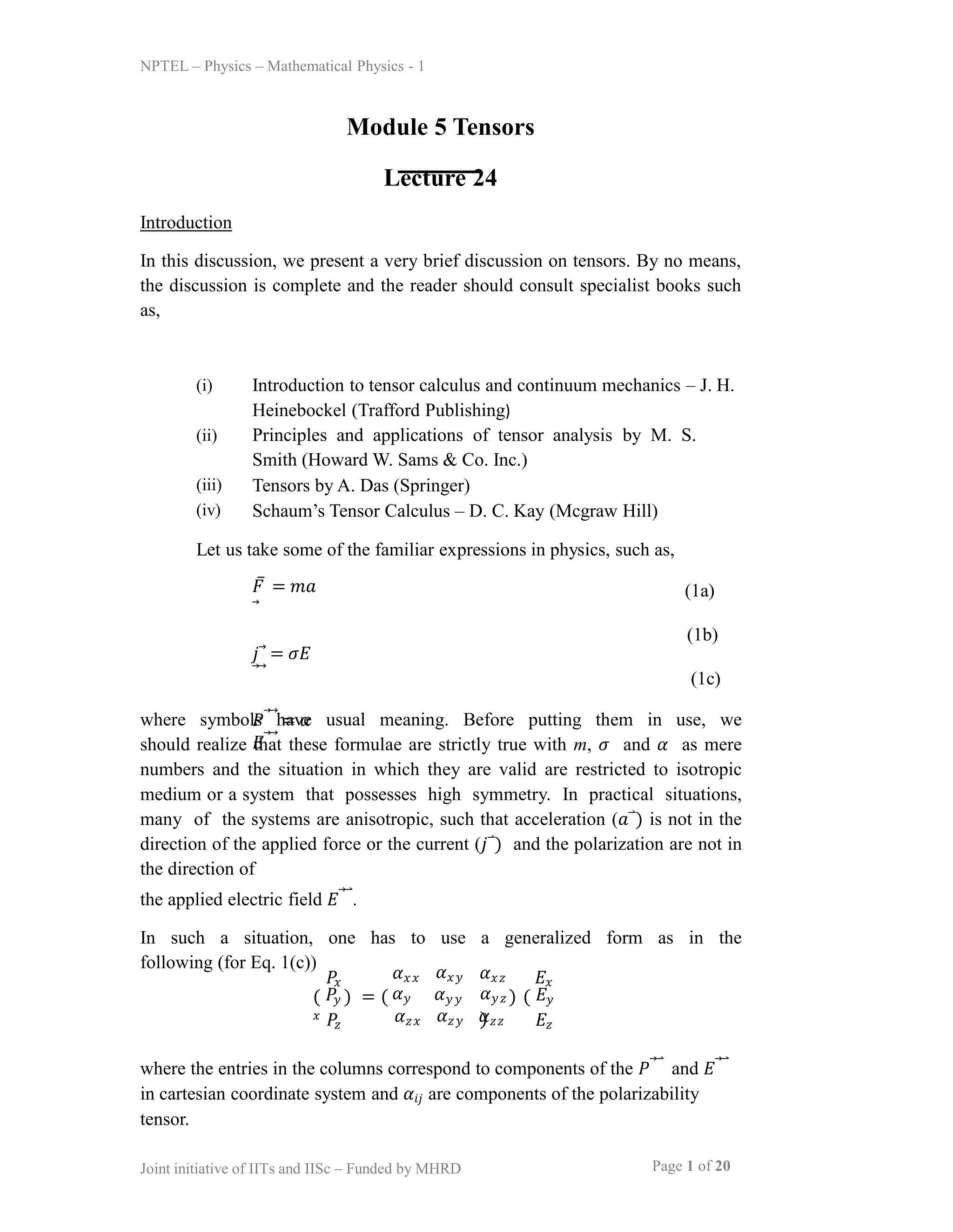
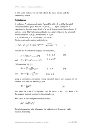
This document provides an introduction to tensors. It discusses that familiar physics equations like F=ma are only strictly true for isotropic systems, and more general tensor forms are needed for anisotropic systems. It gives the example of a polarizability tensor to relate polarization and electric field for an anisotropic medium. It also discusses preliminaries of tensors, including how coordinate transformations define tensors and the Kronecker delta and Levi-Civita tensors used to represent identities and cross products.

1. NPTEL – Physics – Mathematical Physics - 1
Module 5 Tensors
Lecture 24
Introduction
In this discussion, we present a very brief discussion on tensors. By no means,
the discussion is complete and the reader should consult specialist books such
as,
Page 1 of 20
Joint initiative of IITs and IISc – Funded by MHRD
(i) Introduction to tensor calculus and continuum mechanics – J. H.
Heinebockel (Trafford Publishing)
Principles and applications of tensor analysis by M. S.
Smith (Howard W. Sams & Co. Inc.)
Tensors by A. Das (Springer)
Schaum’s Tensor Calculus – D. C. Kay (Mcgraw Hill)
(ii)
(iii)
(iv)
Let us take some of the familiar expressions in physics, such as,
𝐹̅ = 𝑚𝑎
⃗
𝑗⃗ = 𝜎𝐸
⃗⃗
𝑃⃗⃗ = 𝛼
𝐸⃗⃗
(1a)
(1b)
(1c)
where symbols have usual meaning. Before putting them in use, we
should realize that these formulae are strictly true with m, 𝜎 and 𝛼 as mere
numbers and the situation in which they are valid are restricted to isotropic
medium or a system that possesses high symmetry. In practical situations,
many of the systems are anisotropic, such that acceleration (𝑎⃑) is not in the
direction of the applied force or the current (𝑗⃑) and the polarization are not in
the direction of
the applied electric field 𝐸⃗⃑.
In such a situation, one has to use a generalized form as in the
following (for Eq. 1(c))
( 𝑃𝑦 ) = ( 𝛼𝑦
𝑥
𝑃
𝑥
𝑃
𝑧
𝛼𝑧𝑥 𝛼𝑧𝑧 𝐸𝑧
𝛼𝑥𝑥 𝛼𝑥𝑦
𝛼𝑦𝑦
𝛼𝑧𝑦
𝛼𝑥𝑧
𝛼𝑦𝑧 ) ( 𝐸𝑦
)
𝐸𝑥
where the entries in the columns correspond to components of the 𝑃⃗⃑ and 𝐸⃗⃑
in cartesian coordinate system and 𝛼𝑖𝑗 are components of the polarizability
tensor.

2. NPTEL – Physics – Mathematical Physics - 1
In the same fashion we can talk about the mass tensor and the
conductivity tensor.
Preliminaries
If we have a N- dimensional space, 𝑉𝑁 , and let 𝑥𝑖(𝑖 = 1 … 𝑁) be the set of
coordinates in this space. Also let 𝑥̅ 𝛼(𝛼 = 1, … … . 𝑁) be another set of
coordinate in the same space. Each of 𝑥𝑖 𝑠 will depend on the N coordinates 𝑥̅𝛼
and vice versa. The Cartesian coordinates (x, y, z) are related to the spherical
polar coordinates (𝑟, 𝜃, 𝜙), both defined in 𝑉3 as,
𝑥 = 𝑟𝑠𝑖𝑛𝜃𝑐𝑜𝑠𝜙, 𝑦 = 𝑟𝑠𝑖𝑛𝜃𝑠𝑖𝑛𝜙, 𝑧 = 𝑟𝑐𝑜𝑠𝜃.
The inverse transformation is of the form,
r = √𝑥2 + 𝑦2 + 𝑧2, 𝜃 = 𝑡𝑎𝑛−1 (√𝑥2+𝑦2
) , 𝜑 = 𝑡𝑎𝑛−1 (𝑦
)
𝑧 𝑥
Thus for the N- dimensional space, one can define,
𝑥𝑖 = 𝑥𝑖(𝑥̅1, 𝑥̅2 … … … 𝑥̅𝑁)
and 𝑥̅𝛼 = 𝑥̅𝛼(𝑥1, 𝑥2 … … … . 𝑥𝑁)
Differentiation Eq. (1)
1 ≤ 𝑖 ≤ 𝑁 (1)
1 ≤ 𝛼 ≤ 𝑁
𝑑𝑥𝑖 = ∑𝑁 𝜕𝑥𝑖
𝛼=1 𝜕𝑥−𝛼 𝑑𝑥−𝛼 1 ≤ 𝑖 ≤ 𝑁 (2)
and 𝑑𝑥−𝛼 = ∑𝑁 𝜕𝑥−𝛼
𝑖=1 𝜕𝑥
𝑖
𝑑𝑥𝑖
1 ≤ 𝛼 ≤ 𝑁
using a summation convention where repeated indices are assumed to be
summed over, one can write Eq. (2) as,
𝑑𝑥𝑖 = 𝜕𝑥
𝑑𝑥̅𝛼
𝑖
𝜕𝑥̅𝛼 (3)
The above is a set of N equation, one for each i = (1……N). Since 𝛼 is
the repeated index, it assumed to be summed over.
Also since 𝑥𝑖 s are independent of each other,
𝑑𝑥
𝑖
𝑑𝑥𝑗 = {0 for 𝑖 ≠ 𝑗
Page 2 of 20
Joint initiative of IITs and IISc – Funded by MHRD
1 for 𝑖 = 𝑗
The above equation also illustrates the definition of Kronecker delta
function defined by

3. NPTEL – Physics – Mathematical Physics - 1
1 if i,j,k are cyclic
= -1 if i,j,k are counter clockwise
= 0 otherwise
𝛿 = {
𝑗
𝑖 1 if 𝑖 ≠ 𝑗
0 if 𝑖 ≠ 𝑗
Thus
𝑑𝑥
𝑖
𝑑𝑥
𝑗
= 𝛿
𝑗
𝑖
Similarly for the barred coordinates,
𝑑𝑥̅𝛼
𝑑𝑥̅ 𝛽
= 𝛿 thus if {𝑥̅𝛼, 𝑥̅𝛽, 𝑥̅𝛾 … … … . } are independent variables, then
𝛽
𝛼 ,
𝑑𝑥̅𝛼
𝑑𝑥𝛽 is the Kronecker delta, 𝛿𝛽 . The Kronecker delta corresponds to the identity
matrix. Since there are two free indices, it is a second rank tensor.
Page 3 of 20
Joint initiative of IITs and IISc – Funded by MHRD
𝛼
Similarly a third order Levi-Civita tensor is defined as,
1 if 𝑖, 𝑗, 𝑘 are cyclic
𝜀𝑖𝑗𝑘 {= −1 if 𝑖, 𝑗, 𝑘 are counter clockwise
= 0 otherwise
The vector cross product is devoted using the Levi-Civita tensor as,
𝐴⃗ ×
𝐵⃗⃗
= 𝜀𝑖𝑗𝑘 𝐴𝑗 𝐵
𝑘