This document contains the contents and chapter outlines for a book on electromagnetic field theory. It covers topics such as Maxwell's equations, constitutive relations, plane waves, transmission lines, and interactions at material interfaces. The book is intended as lecture notes for a fall 2019 course on electromagnetics at Purdue University, and is continually being updated by the author Weng Cho Chew.


![Lecture 1
Introduction, Maxwell’s
Equations
1.1 Importance of Electromagnetics
We will explain why electromagnetics is so important, and its impact on very many different
areas. Then we will give a brief history of electromagnetics, and how it has evolved in the
modern world. Then we will go briefly over Maxwell’s equations in their full glory. But we
will begin the study of electromagnetics by focussing on static problems.
The discipline of electromagnetic field theory and its pertinent technologies is also known
as electromagnetics. It has been based on Maxwell’s equations, which are the result of the
seminal work of James Clerk Maxwell completed in 1865, after his presentation to the British
Royal Society in 1864. It has been over 150 years ago now, and this is a long time compared
to the leaps and bounds progress we have made in technological advancements. But despite,
research in electromagnetics has continued unabated despite its age. The reason is that
electromagnetics is extremely useful, and has impacted a large sector of modern technologies.
To understand why electromagnetics is so useful, we have to understand a few points
about Maxwell’s equations.
• First, Maxwell’s equations are valid over a vast length scale from subatomic dimensions
to galactic dimensions. Hence, these equations are valid over a vast range of wavelengths,
going from static to ultra-violet wavelengths.1
• Maxwell’s equations are relativistic invariant in the parlance of special relativity [1]. In
fact, Einstein was motivated with the theory of special relativity in 1905 by Maxwell’s
equations [2]. These equations look the same, irrespective of what inertial reference
frame one is in.
• Maxwell’s equations are valid in the quantum regime, as it was demonstrated by Paul
Dirac in 1927 [3]. Hence, many methods of calculating the response of a medium to
1Current lithography process is working with using ultra-violet light with a wavelength of 193 nm.
1](https://image.slidesharecdn.com/emftall20191204-240115133321-d13ecad1/85/EMFTAll2-15-320.jpg)
![2 Electromagnetic Field Theory
classical field can be applied in the quantum regime also. When electromagnetic theory
is combined with quantum theory, the field of quantum optics came about. Roy Glauber
won a Nobel prize in 2005 because of his work in this area [4].
• Maxwell’s equations and the pertinent gauge theory has inspired Yang-Mills theory
(1954) [5], which is also known as a generalized electromagnetic theory. Yang-Mills
theory is motivated by differential forms in differential geometry [6]. To quote from
Misner, Thorne, and Wheeler, “Differential forms illuminate electromagnetic theory,
and electromagnetic theory illuminates differential forms.” [7,8]
• Maxwell’s equations are some of the most accurate physical equations that have been
validated by experiments. In 1985, Richard Feynman wrote that electromagnetic theory
has been validated to one part in a billion.2
Now, it has been validated to one part in
a trillion (Aoyama et al, Styer, 2012).3
• As a consequence, electromagnetics has had a tremendous impact in science and tech-
nology. This is manifested in electrical engineering, optics, wireless and optical commu-
nications, computers, remote sensing, bio-medical engineering etc.
Figure 1.1: The impact of electromagnetics in many technologies. The areas in blue are
prevalent areas impacted by electromagnetics some 20 years ago [9], and the areas in red are
modern emerging areas impacted by electromagnetics.
2This means that if a jet is to fly from New York to Los Angeles, an error of one part in a billion means
an error of a few millmeters.
3This means an error of a hairline, if one were to fly from the earth to the moon.](https://image.slidesharecdn.com/emftall20191204-240115133321-d13ecad1/85/EMFTAll2-16-320.jpg)
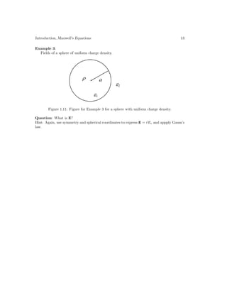
![Introduction, Maxwell’s Equations 3
1.1.1 A Brief History of Electromagnetics
Electricity and magnetism have been known to humans for a long time. Also, the physical
properties of light has been known. But electricity and magnetism, now termed electromag-
netics in the modern world, has been thought to be governed by different physical laws as
opposed to optics. This is understandable as the physics of electricity and magnetism is quite
different of the physics of optics as they were known to humans.
For example, lode stone was known to the ancient Greek and Chinese around 600 BC
to 400 BC. Compass was used in China since 200 BC. Static electricity was reported by
the Greek as early as 400 BC. But these curiosities did not make an impact until the age
of telegraphy. The coming about of telegraphy was due to the invention of the voltaic cell
or the galvanic cell in the late 1700’s, by Luigi Galvani and Alesandro Volta [10]. It was
soon discovered that two pieces of wire, connected to a voltaic cell, can be used to transmit
information.
So by the early 1800’s this possibility had spurred the development of telegraphy. Both
André-Marie Ampére (1823) [11, 12] and Michael Faraday (1838) [13] did experiments to
better understand the properties of electricity and magnetism. And hence, Ampere’s law and
Faraday law are named after them. Kirchhoff voltage and current laws were also developed
in 1845 to help better understand telegraphy [14, 15]. Despite these laws, the technology of
telegraphy was poorly understood. It was not known as to why the telegraphy signal was
distorted. Ideally, the signal should be a digital signal switching between one’s and zero’s,
but the digital signal lost its shape rapidly along a telegraphy line.4
It was not until 1865 that James Clerk Maxwell [17] put in the missing term in Ampere’s
law, the term that involves displacement current, only then the mathematical theory for
electricity and magnetism was complete. Ampere’s law is now known as generalized Ampere’s
law. The complete set of equations are now named Maxwell’s equations in honor of James
Clerk Maxwell.
The rousing success of Maxwell’s theory was that it predicted wave phenomena, as they
have been observed along telegraphy lines. Heinrich Hertz in 1888 [18] did experiment to
proof that electromagnetic field can propagate through space across a room. Moreover, from
experimental measurement of the permittivity and permeability of matter, it was decided
that electromagnetic wave moves at a tremendous speed. But the velocity of light has been
known for a long while from astronomical observations (Roemer, 1676) [19]. The observation
of interference phenomena in light has been known as well. When these pieces of information
were pieced together, it was decided that electricity and magnetism, and optics, are actually
governed by the same physical law or Maxwell’s equations. And optics and electromagnetics
are unified into one field.
4As a side note, in 1837, Morse invented the Morse code for telegraphy [16]. There were cross pollination
of ideas across the Atlantic ocean despite the distance. In fact, Benjamin Franklin associated lightning with
electricity in the latter part of the 18-th century. Also, notice that electrical machinery was invented in 1832
even though electromagnetic theory was not fully understood.](https://image.slidesharecdn.com/emftall20191204-240115133321-d13ecad1/85/EMFTAll2-17-320.jpg)
![4 Electromagnetic Field Theory
Figure 1.2: A brief history of electromagnetics and optics as depicted in this figure.
In Figure 1.2, a brief history of electromagnetics and optics is depicted. In the beginning,
it was thought that electricity and magnetism, and optics were governed by different physical
laws. Low frequency electromagnetics was governed by the understanding of fields and their
interaction with media. Optical phenomena were governed by ray optics, reflection and
refraction of light. But the advent of Maxwell’s equations in 1865 reveal that they can be
unified by electromagnetic theory. Then solving Maxwell’s equations becomes a mathematical
endeavor.
The photo-electric effect [20, 21], and Planck radiation law [22] point to the fact that
electromagnetic energy is manifested in terms of packets of energy. Each unit of this energy
is now known as the photon. A photon carries an energy packet equal to ω, where ω is the
angular frequency of the photon and = 6.626 × 10⁻³⁴
J s, the Planck constant, which is
a very small constant. Hence, the higher the frequency, the easier it is to detect this packet
of energy, or feel the graininess of electromagnetic energy. Eventually, in 1927 [3], quantum
theory was incorporated into electromagnetics, and the quantum nature of light gives rise to
the field of quantum optics. Recently, even microwave photons have been measured [23]. It
is a difficult measurement because of the low frequency of microwave (109
Hz) compared to
optics (1015
Hz): microwave photon has a packet of energy about a million times smaller than
that of optical photon.
The progress in nano-fabrication [24] allows one to make optical components that are
subwavelength as the wavelength of blue light is about 450 nm. As a result, interaction of
light with nano-scale optical components requires the solution of Maxwell’s equations in its
full glory.](https://image.slidesharecdn.com/emftall20191204-240115133321-d13ecad1/85/EMFTAll2-18-320.jpg)
![Introduction, Maxwell’s Equations 5
In 1980s, Bell’s theorem (by John Steward Bell) [25] was experimentally verified in favor of
the Copenhagen school of quantum interpretation (led by Niel Bohr) [26]. This interpretation
says that a quantum state is in a linear superposition of states before a measurement. But
after a measurement, a quantum state collapses to the state that is measured. This implies
that quantum information can be hidden in a quantum state. Hence, a quantum particle,
such as a photon, its state can remain incognito until after its measurement. In other words,
quantum theory is “spooky”. This leads to growing interest in quantum information and
quantum communication using photons. Quantum technology with the use of photons, an
electromagnetic quantum particle, is a subject of growing interest.
1.2 Maxwell’s Equations in Integral Form
Maxwell’s equations can be presented as fundamental postulates.5
We will present them in
their integral forms, but will not belabor them until later.
C
E · dl = −
d
dt
S
B · dS Faraday’s Law (1.2.1)
C
H · dl =
d
dt
S
D · dS + I Ampere’s Law (1.2.2)
S
D · dS = Q Gauss’s or Coulomb’s Law (1.2.3)
S
B · dS = 0 Gauss’s Law (1.2.4)
The units of the basic quantities above are given as:
E: V/m H: A/m
D: C/m2
B: Webers/m2
I: A Q: Coulombs
1.3 Static Electromagnetics
1.3.1 Coulomb’s Law (Statics)
This law, developed in 1785 [27], expresses the force between two charges q1 and q2. If these
charges are positive, the force is repulsive and it is given by
f1→2 =
q1q2
4πεr2
r̂12 (1.3.1)
5Postulates in physics are similar to axioms in mathematics. They are assumptions that need not be
proved.](https://image.slidesharecdn.com/emftall20191204-240115133321-d13ecad1/85/EMFTAll2-19-320.jpg)
![6 Electromagnetic Field Theory
Figure 1.3: The force between two charges q1 and q2. The force is repulsive if the two charges
have the same sign.
f (force): newton
q (charge): coulombs
ε (permittivity): farads/meter
r (distance between q1 and q2): m
r̂12= unit vector pointing from charge 1 to charge 2
r̂12 =
r2 − r1
|r2 − r1|
, r = |r2 − r1| (1.3.2)
Since the unit vector can be defined in the above, the force between two charges can also be
rewritten as
f1→2 =
q1q2(r2 − r1)
4πε|r2 − r1|3
, (r1, r2 are position vectors) (1.3.3)
1.3.2 Electric Field E (Statics)
The electric field E is defined as the force per unit charge [28]. For two charges, one of charge
q and the other one of incremental charge ∆q, the force between the two charges, according
to Coulomb’s law (1.3.1), is
f =
q∆q
4πεr2
r̂ (1.3.4)
where r̂ is a unit vector pointing from charge q to the incremental charge ∆q. Then the force
per unit charge is given by
E =
f
q
, (V/m) (1.3.5)
This electric field E from a point charge q at the orgin is hence
E =
q
4πεr2
r̂ (1.3.6)](https://image.slidesharecdn.com/emftall20191204-240115133321-d13ecad1/85/EMFTAll2-20-320.jpg)
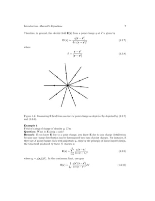
![8 Electromagnetic Field Theory
Figure 1.5: Electric field of a ring of charge (Courtesy of Ramo, Whinnery, and Van Duzer)
[29].
In other words, the total field, by the principle of linear superposition, is the integral sum-
mation of the contributions from the distributed charge density (r).](https://image.slidesharecdn.com/emftall20191204-240115133321-d13ecad1/85/EMFTAll2-22-320.jpg)
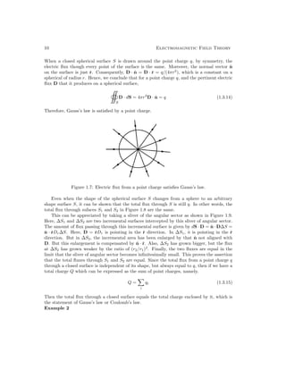
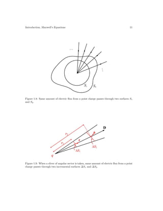
![Introduction, Maxwell’s Equations 9
1.3.3 Gauss’s Law (Statics)
This law is also known as Coulomb’s law as they are closely related to each other. Apparently,
this simple law was first expressed by Joseph Louis Lagrange [30] and later, reexpressed by
Gauss in 1813 (wikipedia).
This law can be expressed as
S
D · dS = Q (1.3.11)
D: electric flux density C/m2
D = εE.
dS: an incremental surface at the point on S given by dSn̂ where n̂ is the unit normal
pointing outward away from the surface.
Q: total charge enclosed by the surface S.
Figure 1.6: Electric flux (Courtesy of Ramo, Whinnery, and Van Duzer) [29]
The left-hand side of (1.3.11) represents a surface integral over a closed surface S. To
understand it, one can break the surface into a sum of incremental surfaces ∆Si, with a
local unit normal n̂i associated with it. The surface integral can then be approximated by a
summation
S
D · dS ≈
i
Di · n̂i∆Si =
i
Di · ∆Si (1.3.12)
where one has defined ∆Si = n̂i∆Si. In the limit when ∆Si becomes infinitesimally small,
the summation becomes a surface integral.
1.3.4 Derivation of Gauss’s Law from Coulomb’s Law (Statics)
From Coulomb’s law and the ensuing electric field due to a point charge, the electric flux is
D = εE =
q
4πr2
r̂ (1.3.13)](https://image.slidesharecdn.com/emftall20191204-240115133321-d13ecad1/85/EMFTAll2-23-320.jpg)

![Lecture 2
Maxwell’s Equations,
Differential Operator Form
2.1 Gauss’s Divergence Theorem
The divergence theorem is one of the most important theorems in vector calculus [29,31–33]
First, we will need to prove Gauss’s divergence theorem, namely, that:
V
dV ∇ · D =
S
D · dS (2.1.1)
In the above, ∇ · D is defined as
∇ · D = lim
∆V →0
∆S
D · dS
∆V
(2.1.2)
and eventually, we will find an expression for it. We know that if ∆V ≈ 0 or small, then the
above,
∆V ∇ · D ≈
∆S
D · dS (2.1.3)
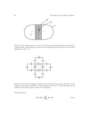
First, we assume that a volume V has been discretized1
into a sum of small cuboids, where
the i-th cuboid has a volume of ∆Vi as shown in Figure 2.1. Then
V ≈
N
X
i=1
∆Vi (2.1.4)
1Other terms are “tesselated”, “meshed”, or “gridded”.
15](https://image.slidesharecdn.com/emftall20191204-240115133321-d13ecad1/85/EMFTAll2-29-320.jpg)
![18 Electromagnetic Field Theory
Factoring out the volume of the cuboid ∆V = ∆x∆y∆z in the above, one gets
∆S
D · dS ≈ ∆V {[Dx(x0 + ∆x, . . .) − Dx(x0, . . .)] /∆x
+ [Dy(. . . , y0 + ∆y, . . .) − Dy(. . . , y0, . . .)] /∆y
+ [Dz(. . . , z0 + ∆z) − Dz(. . . , z0)] /∆z} (2.1.9)
Or that
D · dS
∆V
≈
∂Dx
∂x
+
∂Dy
∂y
+
∂Dz
∂z
(2.1.10)
In the limit when ∆V → 0, then
lim
∆V →0
D · dS
∆V
=
∂Dx
∂x
+
∂Dy
∂y
+
∂Dz
∂z
= ∇ · D (2.1.11)
where
∇ = x̂
∂
∂x
+ ŷ
∂
∂y
+ ẑ
∂
∂z
(2.1.12)
D = x̂Dx + ŷDy + ẑDz (2.1.13)
The divergence operator ∇· has its complicated representations in cylindrical and spherical
coordinates, a subject that we would not delve into in this course. But they are best looked
up at the back of some textbooks on electromagnetics.
Consequently, one gets Gauss’s divergence theorem given by
V
dV ∇ · D =
S
D · dS (2.1.14)
2.1.1 Gauss’s Law in Differential Operator Form
By further using Gauss’s or Coulomb’s law implies that
S
D · dS = Q =
dV % (2.1.15)
which is equivalent to
V
dV ∇ · D =
V
dV % (2.1.16)
When V → 0, we arrive at the pointwise relationship, a relationship at a point in space:
∇ · D = % (2.1.17)](https://image.slidesharecdn.com/emftall20191204-240115133321-d13ecad1/85/EMFTAll2-32-320.jpg)
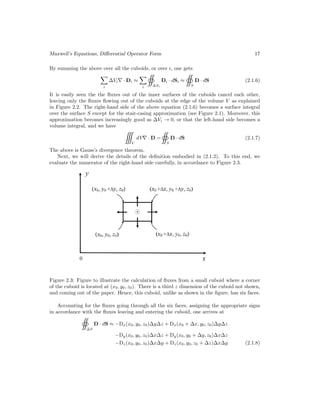
![Maxwell’s Equations, Differential Operator Form 19
2.1.2 Physical Meaning of Divergence Operator
The physical meaning of divergence is that if ∇·D = 0 at a point in space, it implies that there
are fluxes oozing or exuding from that point in space [34]. On the other hand, if ∇ · D = 0,
if implies no flux oozing out from that point in space. In other words, whatever flux that
goes into the point must come out of it. The flux is termed divergence free. Thus, ∇ · D is a
measure of how much sources or sinks exists for the flux at a point. The sum of these sources
or sinks gives the amount of flux leaving or entering the surface that surrounds the sources
or sinks.
Moreover, if one were to integrate a divergence-free flux over a volume V , and invoking
Gauss’s divergence theorem, one gets
S
D · dS = 0 (2.1.18)
In such a scenerio, whatever flux that enters the surface S must leave it. In other words, what
comes in must go out of the volume V , or that flux is conserved. This is true of incompressible
fluid flow, electric flux flow in a source free region, as well as magnetic flux flow, where the
flux is conserved.
Figure 2.4: In an incompressible flux flow, flux is conserved: whatever flux that enters a
volume V must leave the volume V .
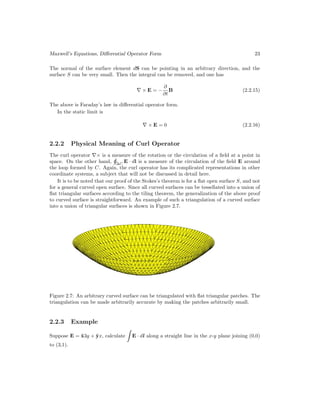
2.1.3 Example
If D = (2y2
+ z)x̂ + 4xyŷ + xẑ, find:
1. Volume charge density ρv at (−1, 0, 3).
2. Electric flux through the cube defined by
0 ≤ x ≤ 1, 0 ≤ y ≤ 1, 0 ≤ z ≤ 1.
3. Total charge enclosed by the cube.](https://image.slidesharecdn.com/emftall20191204-240115133321-d13ecad1/85/EMFTAll2-33-320.jpg)
![20 Electromagnetic Field Theory
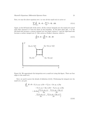
2.2 Stokes’s Theorem
The mathematical description of fluid flow was well established before the establishment of
electromagnetic theory [35]. Hence, much mathematical description of electromagnetic theory
uses the language of fluid. In mathematical notations, Stokes’s theorem is
C
E · dl =
S
∇ × E · dS (2.2.1)
In the above, the contour C is a closed contour, whereas the surface S is not closed.2
First, applying Stokes’s theorem to a small surface ∆S, we define a curl operator 3
∇×
at a point to be
∇ × E · n̂ = lim
∆S→0
∆C
E · dl
∆S
(2.2.2)
Figure 2.5: In proving Stokes’s theorem, a closed contour C is assumed to enclose an open
surface S. Then the surface S is tessellated into sum of small rects as shown. Stair-casing
error vanishes in the limit when the rects are made vanishingly small.
First, the surface S enclosed by C is tessellated into sum of small rects (rectangles).
Stokes’s theorem is then applied to one of these small rects to arrive at
∆Ci
Ei · dli = (∇ × Ei) · ∆Si (2.2.3)
2In other words, C has no boundary whereas S has boundary. A closed surface S has no boundary like
when we were proving Gauss’s divergence theorem previously.
3Sometimes called a rotation operator.](https://image.slidesharecdn.com/emftall20191204-240115133321-d13ecad1/85/EMFTAll2-34-320.jpg)
![Lecture 3
Constitutive Relations, Wave
Equation, Electrostatics, and
Static Green’s Function
3.1 Simple Constitutive Relations
The constitution relation between D and E in free space is
D = ε0E (3.1.1)
When material medium is present, one has to add the contribution to D by the polarization
density P which is a dipole density.1
Then [29,31,36]
D = ε0E + P (3.1.2)
The second term above is the contribution to the electric flux due to the polarization density
of the medium. It is due to the little dipole contribution due to the polar nature of the atoms
or molecules that make up a medium.
By the same token, the first term ε0E can be thought of as the polarization density
contribution of vacuum. Vacuum, though represents nothingness, has electrons and positrons,
or electron-positron pairs lurking in it [37]. Electron is matter, whereas positron is anti-
matter. In the quiescent state, they represent nothingness, but they can be polarized by an
electric field E. That also explains why electromagnetic wave can propagate through vacuum.
For many media, it can be assumed to be a linear media. Then P = ε0χ0E
D = ε0E + ε0χ0E
= ε0(1 + χ0)E = εE (3.1.3)
1Note that a dipole moment is given by Q` where Q is its charge in coulomb and ` is its length in m. Hence,
dipole density, or polarization density as dimension of coulomb/m2, which is the same as that of electric flux
D.
25](https://image.slidesharecdn.com/emftall20191204-240115133321-d13ecad1/85/EMFTAll2-39-320.jpg)
![26 Electromagnetic Field Theory
where χ0 is the electric susceptibility. In other words, for linear material media, one can
replace the vacuum permittivity ε0 with an effective permittivity ε.
In free space:
ε = ε0 = 8.854 × 10⁻¹²
≈
10−8
36π
F/m (3.1.4)
The constitutive relation between magnetic flux B and magnetic field H is given as
B = µH, µ = permeability H/m (3.1.5)
In free space,
µ = µ0 = 4π × 10−7
H/m (3.1.6)
As shall be explained later, this is an assigned value. In other materials, the permeability can
be written as
µ = µ0µr (3.1.7)
Similarly, the permittivity for electric field can be written as
ε = ε0εr (3.1.8)
In the above, µr and εr are relative permeability and relative permeability.
3.2 Emergence of Wave Phenomenon, Triumph of Maxwell’s
Equations
One of the major triumphs of Maxwell’s equations is the prediction of the wave phenomenon.
This was experimentally verified by Heinrich Hertz in 1888 [18], some 23 years after the com-
pletion of Maxwell’s theory [17]. Then it was realized that electromagnetic wave propagates
at a tremendous velocity which is the velocity of light. This was also the defining moment
which revealed that the field of electricity and magnetism and the field of optics were both
described by Maxwell’s equations or electromagnetic theory.
To see this, we consider the first two Maxwell’s equations for time-varying fields in vacuum
or a source-free medium.2
They are
∇ × E = −µ0
∂H
∂t
(3.2.1)
∇ × H = −ε0
∂E
∂t
(3.2.2)
Taking the curl of (3.2.1), we have
∇ × ∇ × E = −µ0
∂
∂t
∇ × H (3.2.3)
2Since the third and the fourth Maxwell’s equations are derivable from the first two.](https://image.slidesharecdn.com/emftall20191204-240115133321-d13ecad1/85/EMFTAll2-40-320.jpg)
![Constitutive Relations, Wave Equation, Electrostatics, and Static Green’s Function 27
It is understood that in the above, the double curl operator implies ∇×(∇×E). Substituting
(3.2.2) into (3.2.3), we have
∇ × ∇ × E = −µ0ε0
∂2
∂t2
E (3.2.4)
In the above, the left-hand side can be simplified by using the identity that a × (b × c) =
b(a · c) − c(a · b),3
but be mindful that the operator ∇ has to operate on a function to its
right. Therefore, we arrive at the identity that
∇ × ∇ × E = ∇∇ · E − ∇2
E (3.2.5)
and that ∇ · E = 0 in a source-free medium, we have
∇2
E − µ0ε0
∂2
∂t2
E = 0 (3.2.6)
where
∇2
= ∇ · ∇ =
∂2
∂x2
∂2
∂x2
+
∂2
∂y2
+
∂2
∂z2
Here, (3.2.6) is the wave equation in three space dimensions [31,38].
To see the simplest form of wave emerging in the above, we can let E = x̂Ex(z, t) so that
∇ · E = 0 satisfying the source-free condition. Then (3.2.6) becomes
∂2
∂z2
Ex(z, t) − µ0ε0
∂2
∂t2
Ex(z, t) = 0 (3.2.7)
Eq. (3.2.7) is known mathematically as the wave equation in one space dimension. It can
also be written as
∂2
∂z2
f(z, t) −
1
c2
0
∂2
∂t2
f(z, t) = 0 (3.2.8)
where c2
0 = (µ0ε0)−1
. Eq. (3.2.8) can also be factorized as
∂
∂z
−
1
c0
∂
∂t
∂
∂z
+
1
c0
∂
∂t
f(z, t) = 0 (3.2.9)
or
∂
∂z
+
1
c0
∂
∂t
∂
∂z
−
1
c0
∂
∂t
f(z, t) = 0 (3.2.10)
The above implies that we have
∂
∂z
+
1
c0
∂
∂t
f+(z, t) = 0 (3.2.11)
3For mnemonics, this formula is also known as the “back-of-the-cab” formula.](https://image.slidesharecdn.com/emftall20191204-240115133321-d13ecad1/85/EMFTAll2-41-320.jpg)
![28 Electromagnetic Field Theory
or
∂
∂z
−
1
c0
∂
∂t
f−(z, t) = 0 (3.2.12)
Equation (3.2.11) and (3.2.12) are known as the one-way wave equations or advective equa-
tions [39]. From the above factorization, it is seen that the solutions of these one-way wave
equations are also the solutions of the original wave equation given by (3.2.8). Their general
solutions are then
f+(z, t) = F+(z − c0t) (3.2.13)
f−(z, t) = F−(z + c0t) (3.2.14)
Eq. (3.2.13) constitutes a right-traveling wave function of any shape while (3.2.14) constitutes
a left-traveling wave function of any shape. Since Eqs. (3.2.13) and (3.2.14) are also solutions
to (3.2.8), we can write the general solution to the wave equation as
f(z, t) = F+(z − c0t) + F−(z + c0t) (3.2.15)
This is a wonderful result since F+ and F− are arbitrary functions of any shape (see Figure
3.1); they can be used to encode information for communication!
Figure 3.1: Solutions of the wave equation can be a single-valued function of any shape. In
the above, F+ travels in the positive z direction, while F− travels in the negative z direction
as t increases.](https://image.slidesharecdn.com/emftall20191204-240115133321-d13ecad1/85/EMFTAll2-42-320.jpg)
![Constitutive Relations, Wave Equation, Electrostatics, and Static Green’s Function 29
Furthermore, one can calculate the velocity of this wave to be
c0 = 299, 792, 458m/s ' 3 × 10⁸
m/s (3.2.16)
where c0 =
p
1/µ0ε0.
Maxwell’s equations (3.2.1) implies that E and H are linearly proportional to each other.
Thus, there is only one independent constant in the wave equation, and the value of µ0 is
defined to be 4π × 10−7
henry m−1
, while the value of ε0 has been measured to be about
8.854 × 10⁻¹²
farad m−1
. Now it has been decided that the velocity of light is defined to
be the integer given in (3.2.16). A meter is defined to be the distance traveled by light
in 1/(299792458) seconds. Hence, the more accurate that unit of time or second can be
calibrated, the more accurate can we calibrate the unit of length or meter.
3.3 Static Electromagnetics–Revisted
We have seen static electromagnetics previously in integral form. Now we look at them in
differential operator form. When the fields and sources are not time varying, namely that
∂/∂t = 0, we arrive at the static Maxwell’s equations for electrostatics and magnetostatics,
namely [29,31,40]
∇ × E = 0 (3.3.1)
∇ × H = J (3.3.2)
∇ · D = % (3.3.3)
∇ · B = 0 (3.3.4)
Notice the the electrostatic field system is decoupled from the magnetostatic field system.
However, in a resistive system where
J = σE (3.3.5)
the two systems are coupled again. This is known as resistive coupling between them. But if
σ → ∞, in the case of a perfect conductor, or superconductor, then for a finite J, E has to
be zero. The two systems are decoupled again.
Also, one can arrive at the equations above by letting µ0 → 0 and 0 → 0. In this case,
the velocity of light becomes infinite, or retardation effect is negligible. In other words, there
is no time delay for signal propagation through the system in the static approximation.
3.3.1 Electrostatics
We see that Faraday’s law in the static limit is
∇ × E = 0 (3.3.6)
One way to satisfy the above is to let E = −∇Φ because of the identity ∇ × ∇ = 0.4
Alternatively, one can assume that E is a constant. But we usually are interested in solutions
4One an easily go through the algebra to convince oneself of this.](https://image.slidesharecdn.com/emftall20191204-240115133321-d13ecad1/85/EMFTAll2-43-320.jpg)
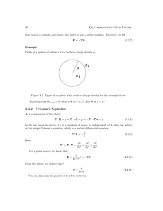
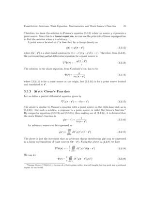
![32 Electromagnetic Field Theory
By substituting the above into the left-hand side of (3.3.18), exchanging order of integration
and differentiation, and then making use of equation (3.3.9), it can be shown that (3.3.19)
indeed satisfies (3.3.11). The above is just a convolutional integral. Hence, the potential Φ(r)
due to an arbitrary source distribution (r) can be found by using convolution, namely,
Φ(r) =
1
4πε V
(r
)
|r − r|
dV
(3.3.20)
In a nutshell, the solution of Poisson’s equation when it is driven by an arbitrary source , is
the convolution of the source with the static Green’s function, a point source response.
3.3.4 Laplace’s Equation
If = 0, or if we are in a source-free region,
∇2
Φ =0 (3.3.21)
which is the Laplace’s equation. Laplace’s equation is usually solved as a boundary value
problem. In such a problem, the potential Φ is stipulated on the boundary of a region, and
then the solution is sought in the intermediate region so as to match the boundary condition.
Examples of such boundary value problems are given below.
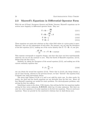
Example 1
A capacitor has two parallel plates attached to a battery, what is E field inside the capacitor?
First, one guess the electric field between the two parallel plates. Then one arrive at a
potential Φ in between the plates so as to produce the field. Then the potential is found so
as to match the boundary conditions of Φ = V in the upper plate, and Φ = 0 in the lower
plate. What is the Φ that will satisfy the requisite boundary condition?
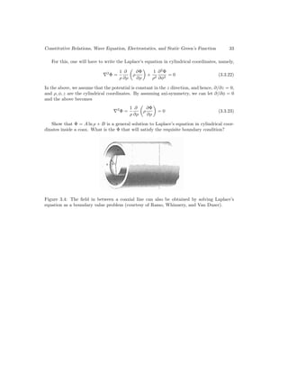
Figure 3.3: Figure of a parallel plate capacitor. The field in between can be found by solving
Laplace’s equation as a boundary value problem [29].
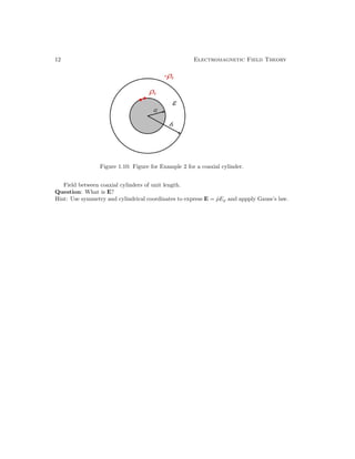
Example 2
A coaxial cable has two conductors. The outer conductor is grounded and hence is at zero
potential. The inner conductor is at voltage V . What is the solution?](https://image.slidesharecdn.com/emftall20191204-240115133321-d13ecad1/85/EMFTAll2-46-320.jpg)

![Lecture 4
Magnetostatics, Boundary
Conditions, and Jump
Conditions
4.1 Magnetostatics
The magnetostatic equations where ∂/∂t = 0 are [29,31,40]
∇ × H = J (4.1.1)
∇ · B = 0 (4.1.2)
One way to satisfy the second equation is to let
B = ∇ × A (4.1.3)
because
∇ · (∇ × A) = 0 (4.1.4)
The above is zero for the same reason that a · (a × b) = 0. In this manner, Gauss’s law is
automatically satisfied.
From (4.1.1), we have
∇ ×
B
µ
= J (4.1.5)
Then using (4.1.3)
∇ ×
1
µ
∇ × A
= J (4.1.6)
35](https://image.slidesharecdn.com/emftall20191204-240115133321-d13ecad1/85/EMFTAll2-49-320.jpg)
![36 Electromagnetic Field Theory
In a homogeneous medium, µ is a constant and hence
∇ × (∇ × A) = µJ (4.1.7)
We use the vector identity that (see previous lecture)
∇ × (∇ × A) = ∇(∇ · A) − (∇ · ∇)A
= ∇(∇ · A) − ∇2
A (4.1.8)
As a result, we arrive at [41]
∇(∇ · A) − ∇2
A = µJ (4.1.9)
By imposing the Coulomb’s gauge that ∇·A = 0, which will be elaborated in the next section,
we arrive at
∇2
A = −µJ (4.1.10)
The above is also known as the vector Poisson’s equation. In cartesian coordinates, the above
can be viewed as three scalar Poisson’s equations. Each of the Poisson’s equation can be
solved using the Green’s function method previously described. Consequently, in free space
A(r) =
µ
4π
V
J(r0
)
R
dV 0
(4.1.11)
where
R = |r − r0
| (4.1.12)
and dV 0
= dx0
dy0
dz0
. It is also variously written as dr0
or d3
r0
.
4.1.1 More on Coulomb’s Gauge
Gauge is a very important concept in physics [42], and we will further elaborate it here. First,
notice that A in (4.1.3) is not unique because one can always define
A0
= A − ∇Ψ (4.1.13)
Then
∇ × A0
= ∇ × (A − ∇Ψ) = ∇ × A = B (4.1.14)
where we have made use of that ∇ × ∇Ψ = 0. Hence, the ∇× of both A and A0
produce the
same B.
To find A uniquely, we have to define or set the divergence of A or provide a gauge
condition. One way is to set the divergence of A to be zero, namely
∇ · A = 0 (4.1.15)](https://image.slidesharecdn.com/emftall20191204-240115133321-d13ecad1/85/EMFTAll2-50-320.jpg)
![Magnetostatics, Boundary Conditions, and Jump Conditions 37
Then
∇ · A0
= ∇ · A − ∇2
Ψ 6= ∇ · A (4.1.16)
The last non-equal sign follows if ∇2
Ψ 6= 0. However, if we further stipulate that ∇ · A0
=
∇ · A = 0, then −∇2
Ψ = 0. This does not necessary imply that Ψ = 0, but if we impose that
condition that Ψ → 0 when r → ∞, then Ψ = 0 everywhere.1
By so doing, A and A0
are
equal to each other, and we obtain (4.1.10) and (4.1.11).
4.2 Boundary Conditions–1D Poisson’s Equation
Boundary conditions are embedded in the partial differential equations that the potential or
the field satisfy. Two important concepts to keep in mind are:
• Differentiation of a function with discontinuous slope will give rise to step discontinuity.
• Differentiation of a function with step discontinuity will give rise to a Dirac delta func-
tion. This is also called the jump condition, a term often used by the mathematics
community [43].
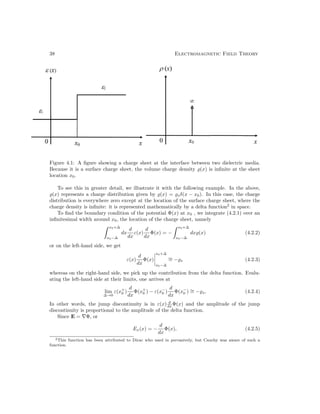
Take for example a one dimensional Poisson’s equation that
d
dx
ε(x)
d
dx
Φ(x) = −%(x) (4.2.1)
where ε(x) represents material property that has the form given in Figure 4.1. One can
actually say a lot about Φ(x) given %(x) on the right-hand side. If %(x) has a delta function
singularity, it implies that ε(x) d
dx Φ(x) has a step discontinuity. If %(x) is finite everywhere,
then ε(x) d
dx Φ(x) must be continuous everywhere.
Furthermore, if ε(x) d
dx Φ(x) is finite everywhere, it implies that Φ(x) must be continuous
everywhere.
1It is a property of the Laplace boundary value problem that if Ψ = 0 on a closed surface S, then Ψ = 0
everywhere inside S. Earnshaw’s theorem is useful for proving this assertion.](https://image.slidesharecdn.com/emftall20191204-240115133321-d13ecad1/85/EMFTAll2-51-320.jpg)
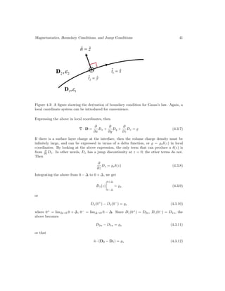
![Magnetostatics, Boundary Conditions, and Jump Conditions 39
The above implies that
ε(x+
0 )Ex(x+
0 ) − ε(x−
0 )Ex(x−
0 ) = s (4.2.6)
or
Dx(x+
0 ) − Dx(x−
0 ) = s (4.2.7)
where
Dx(x) = ε(x)Ex(x) (4.2.8)
The lesson learned from above is that boundary condition is obtained by integrating the
pertinent differential equation over an infinitesimal small segment. In this mathematical
way of looking at the boundary condition, one can also eyeball the differential equation and
ascertain the terms that will have the jump discontinuity that will yield the delta function
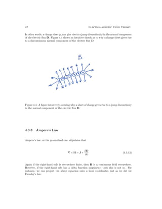
on the right-hand side.
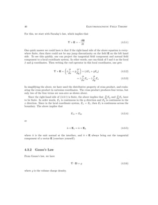
4.3 Boundary Conditions–Maxwell’s Equations
As seen previously, boundary conditions for a field is embedded in the differential equation
that the field satisfies. Hence, boundary conditions can be derived from the differential
operator forms of Maxwell’s equations. In most textbooks, boundary conditions are obtained
by integrating Maxwell’s equations over a small pill box [29,31,41]. To derive these boundary
conditions, we will take an unconventional view: namely to see what sources can induce jump
conditions on the pertinent fields. Boundary conditions are needed at media interfaces, as
well as across current or charge sheets.
4.3.1 Faraday’s Law
Figure 4.2: This figure is for the derivation of Faraday’s law. A local coordinate system can be
used to see the boundary condition more lucidly. Here, the normal n̂ = ŷ and the tangential
component t̂ = x̂.](https://image.slidesharecdn.com/emftall20191204-240115133321-d13ecad1/85/EMFTAll2-53-320.jpg)
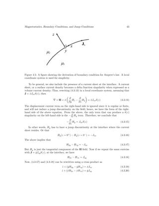
![Lecture 5
Biot-Savart law, Conductive
Media Interface, Instantaneous
Poynting’s Theorem
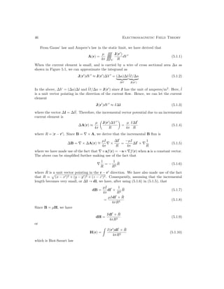
5.1 Derivation of Biot-Savart Law
Figure 5.1: A current element used to illustrate the derivation of Biot-Savart law. The current
element generates a magnetic field due to Ampere’s law in the static limit.
Biot-Savart law, like Ampere’s law was experimentally determined in around 1820 and it
is discussed in a number of textbooks [29, 31, 42]. This is the cumulative work of Ampere,
Oersted, Biot, and Savart. Nowadays, we have the mathematical tool to derive this law from
Ampere’s law and Gauss’s law for magnetostatics.
45](https://image.slidesharecdn.com/emftall20191204-240115133321-d13ecad1/85/EMFTAll2-59-320.jpg)
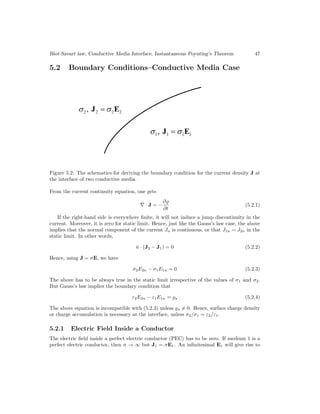
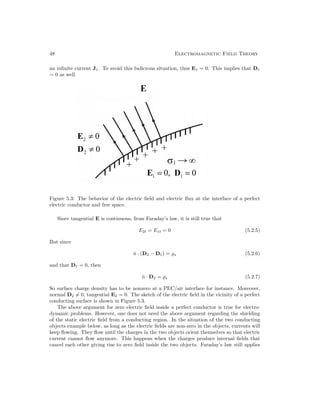
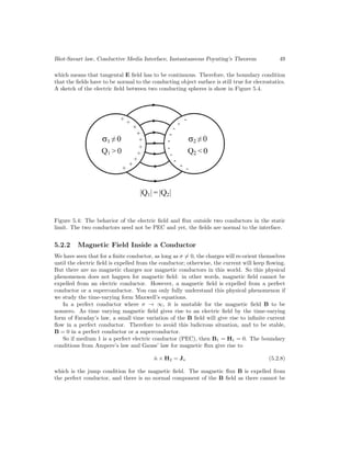
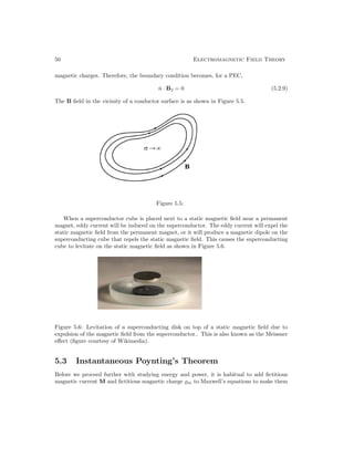
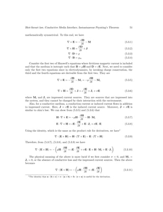
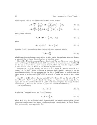
![Biot-Savart law, Conductive Media Interface, Instantaneous Poynting’s Theorem 53
Now, if we let σ 6= 0, then the term to be included is then σE · E = σ|E|2
which has the
unit of S m−1
times V2
m−2
, or W m−3
where S is siemens. We gather this unit by noticing
that 1
2
V 2
R is the power dissipated in a resistor of R ohms with a unit of watts. The reciprocal
unit of ohms, which used to be mhos is now siemens. With σ 6= 0, (5.3.18) becomes
∇ · Sp = −
∂
∂t
Wt − σ|E|2
= −
∂
∂t
We − Pd (5.3.19)
Here, ∇·Sp has physical meaning of power density oozing out from a point, and −Pd = −σ|E|2
has the physical meaning of power density dissipated (siphoned) at a point by the conductive
loss in the medium which is proportional to −σ|E|2
.
Now if we set Ji and Mi to be nonzero, (5.3.19) is augmented by the last two terms in
(5.3.10), or
∇ · Sp = −
∂
∂t
Wt − Pd − H · Mi − E · Ji (5.3.20)
The last two terms can be interpreted as the power density supplied by the impressed currents
Mi and Ji. Hence, (5.3.20) becomes
∇ · Sp = −
∂
∂t
Wt − Pd + Ps (5.3.21)
where
Ps = −H · Mi − E · Ji (5.3.22)
where Ps is the power supplied by the impressed current sources. These terms are positive if
H and Mi have opposite signs, or if E and Ji have opposite signs. The last terms reminds us
of what happens in a negative resistance device or a battery.2
In a battery, positive charges
move from a region of lower potential to a region of higher potential (see Figure 5.7). The
positive charges move from one end of a battery to the other end of the battery. Hence, they
are doing an “uphill climb” due to chemical processes within the battery.
2A negative resistance has been made by Leo Esaki [44], winning him a share in the Nobel prize.](https://image.slidesharecdn.com/emftall20191204-240115133321-d13ecad1/85/EMFTAll2-67-320.jpg)
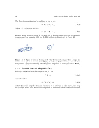
![Lecture 6
Time-Harmonic Fields, Complex
Power
6.1 Time-Harmonic Fields—Linear Systems
The analysis of Maxwell’s equations can be greatly simplified by assuming the fields to be
time harmonic, or sinusoidal (cosinusoidal). Electrical engineers use a method called phasor
technique [31,45], to simplify equations involving time-harmonic signals. This is also a poor-
man’s Fourier transform [46]. That is one begets the benefits of Fourier transform technique
without knowledge of Fourier transform. Since only one time-harmonic frequency is involved,
this is also called frequency domain analysis.1
Figure 6.1: Courtesy of Wikipedia and Pinterest.
1It is simple only for linear systems: for nonlinear systems, such analysis can be quite unwieldy. But rest
assured, as we will not discuss nonlinear systems in this course.
55](https://image.slidesharecdn.com/emftall20191204-240115133321-d13ecad1/85/EMFTAll2-69-320.jpg)
![56 Electromagnetic Field Theory
To learn phasor techniques, one makes use the formula due to Euler (1707–1783) (Wikipedia)
ejα
= cos α + j sin α (6.1.1)
where j =
√
−1 is an imaginary number. But lo and behold, in other disciplines,
√
−1 is
denoted by “i”, but “i” is too close to the symbol for current. So the preferred symbol for
electrical engineering for an imaginary number is j: a quirkness of convention, just as positive
charges do not carry current in a wire.
From Euler’s formula one gets
cos α = e(ejα
) (6.1.2)
Hence, all time harmonic quantity can be written as
V (x, y, z, t) = V 0
(x, y, z) cos(ωt + α) (6.1.3)
= V 0
(r)e(ej(ωt+α)
) (6.1.4)
= e V 0
(r)ejα
ejωt
(6.1.5)
= e
V
e
(r)ejωt
(6.1.6)
Now V
e
(r) = V 0
(r)ejα
is a complex number called the phasor representation or phasor of
V (r, t) a time-harmonic quantity.2
Here, the phase α = α(r) can also be a function of
position r, or x, y, z. Consequently, any component of a field can be expressed as
Ex(x, y, z, t) = Ex(r, t) = e[E
e
x(r)ejωt
] (6.1.7)
The above can be repeated for y and z components. Compactly, one can write
E(r, t) = e[E
e
(r)ejωt
] (6.1.8)
H(r, t) = e[H
e
(r)ejωt
] (6.1.9)
where E
e
and H
e
are complex vector fields. Such phasor representations of time-harmonic fields
simplify Maxwell’s equations. For instance, if one writes
B(r, t) = e
B
e
(r)ejωt
(6.1.10)
then
∂
∂t
B(r, t) =
∂
∂t
e[B
e
(r)ejωt
]
= e
∂
∂t
B
e
(r)jωejωt
= e
B
e
(r)jωejωt
(6.1.11)
2We will use under tilde to denote a complex number or a phasor here, but this notation will be dropped
later. Whether a variable is complex or real is clear from the context.](https://image.slidesharecdn.com/emftall20191204-240115133321-d13ecad1/85/EMFTAll2-70-320.jpg)
![Time-Harmonic Fields, Complex Power 57
Therefore, a time derivative can be effected very simply for a time-harmonic field. One just
needs to multiply jω to the phasor representation of a field or a signal. Therefore, given
Faraday’s law that
∇ × E = −
∂B
∂t
− M (6.1.12)
assuming that all quantities are time harmonic, then
E(r, t) = e[E
e
(r)ejωt
] (6.1.13)
M(r, t) = e[M
f
(r)ejωt
] (6.1.14)
using (6.1.11), and (6.1.14), into (6.1.12), one gets
∇ × E(r, t) = e[∇ × E
e
(r)ejωt
] (6.1.15)
and that
e[∇ × E
e
(r)ejωt
] = −e[B
e
(r)jωejωt
] − e[M
f
(r)ejωt
] (6.1.16)
Since if
e[Aejωt
] = e[B(r)ejωt
], ∀t (6.1.17)
then A = B, it must be true from (6.1.16) that
∇ × E
e
(r) = −jωB
e
(r) − M
f
(r) (6.1.18)
Hence, finding the phasor representation of an equation is clear: whenever we have ∂
∂t , we
replace it by jω. Applying this methodically to the other Maxwell’s equations, we have
∇ × H
e
(r) = jωD
e
(r) + J
e
(r) (6.1.19)
∇ · D
e
(r) = %
e
e(r) (6.1.20)
∇ · B
e
(r) = %
e
m(r) (6.1.21)
In the above, the phasors are functions of frequency. For instance, H
e
(r) should rightly be
written as H
e
(r, ω), but the ω dependence is implied.
6.2 Fourier Transform Technique
In the phasor representation, Maxwell’s equations has no time derivatives; hence the equations
are simplified. We can also arrive at the above simplified equations using Fourier transform](https://image.slidesharecdn.com/emftall20191204-240115133321-d13ecad1/85/EMFTAll2-71-320.jpg)
![Time-Harmonic Fields, Complex Power 59
6.3 Complex Power
Consider now that in the phasor representations, E
e
(r) and H
e
(r) are complex vectors, and
their cross product, E
e
(r) × H
e
∗
(r), which still has the unit of power density, has a different
physical meaning. First, consider the instantaneous Poynting’s vector
S(r, t) = E(r, t) × H(r, t) (6.3.1)
where all the quantities are real valued. Now, we can use phasor technique to analyze the
above. Assuming time-harmonic fields, the above can be rewritten as
S(r, t) = e[E
e
(r)ejωt
] × e[H
e
(r)ejωt
]
=
1
2
[E
e
ejωt
+ (E
e
ejωt
)∗
] ×
1
2
[H
e
ejωt
+ (H
e
ejωt
)∗
] (6.3.2)
where we have made use of the formula that
e(Z) =
1
2
(Z + Z∗
) (6.3.3)
Then more elaborately, on expanding (6.3.2), we get
S(r, t) =
1
4
E
e
× H
e
e2jωt
+
1
4
E
e
× H
e
∗
+
1
4
E
e
∗
× H
e
+
1
4
E
e
∗
× H
e
∗
e−2jωt
(6.3.4)
Then rearranging terms and using (6.3.3) yield
S(r, t) =
1
2
e[E
e
× H
e
∗
] +
1
2
e[E
e
× H
e
e2jωt
] (6.3.5)
where the first term is independent of time, while the second term is sinusoidal in time. If we
define a time-average quantity such that
Sav = hS(r, t)i = lim
T →∞
1
T
T
0
S(r, t)dt (6.3.6)
then it is quite clear that the second term of (6.3.5) time averages to zero, and
Sav = hS(r, t)i =
1
2
e[E
e
× H
e
∗
] (6.3.7)
Hence, in the phasor representation, the quantity
S
e
= E
e
× H
e
(6.3.8)
is termed the complex Poynting’s vector. The power flow associated with it is termed complex
power.](https://image.slidesharecdn.com/emftall20191204-240115133321-d13ecad1/85/EMFTAll2-73-320.jpg)
![60 Electromagnetic Field Theory
Figure 6.2:
To understand what complex power is , it is fruitful if we revisit complex power [47, 48]
in our circuit theory course. The circuit in Figure 6.2 can be easily solved by using phasor
technique. The impedance of the circuit is Z = R + jωL. Hence,
V
= (R + jωL)I
(6.3.9)
where V
and I
are the phasors of the voltage and current for time-harmonic signals. Just as
in the electromagnetic case, the complex power is taken to be
P
= V
I
∗
(6.3.10)
But the instantaneous power is given by
Pinst(t) = V (t)I(t) (6.3.11)
where V (t) = e{V
ejωt
} and I(t) = e{I
ejωt
}. As shall be shown below,
Pav = Pinst(t) =
1
2
e[P
] (6.3.12)
It is clear that if V (t) is sinusoidal, it can be written as
V (t) = V0 cos(ωt) = e[V
ejωt
] (6.3.13)
where, without loss of generality, we assume that V
= V0. Then from (6.3.9), it is clear that
V (t) and I(t) are not in phase. Namely that
I(t) = I0 cos(ωt + α) = e[I
ejωt
] (6.3.14)
where I
= I0ejα
. Then
Pinst(t) = V0I0 cos(ωt) cos(ωt + α)
= V0I0 cos(ωt)[cos(ωt) cos(α) − sin(ωt) sin α]
= V0I0 cos2
(ωt) cos α − V0I0 cos(ωt) sin(ωt) sin α (6.3.15)](https://image.slidesharecdn.com/emftall20191204-240115133321-d13ecad1/85/EMFTAll2-74-320.jpg)
![Time-Harmonic Fields, Complex Power 61
It can be seen that the first term does not time-average to zero, but the second term does.
Now taking the time average of (6.3.15), we get
Pav = Pinst =
1
2
V0I0 cos α =
1
2
e[V
I
∗
] (6.3.16)
=
1
2
e[P
] (6.3.17)
On the other hand, the reactive power
Preactive =
1
2
m[P
] =
1
2
m[V
I
∗
] =
1
2
m[V0I0e−jα
] = −
1
2
V0I0 sin α (6.3.18)
One sees that amplitude of the time-varying term in (6.3.15) is precisely proportional to
m[P
].3
The reason for the existence of imaginary part of P
is because V (t) and I(t) are out of
phase or V
= V0, but I
= I0ejα
. The reason why they are out of phase is because the circuit
has a reactive part to it. Hence the imaginary part of complex power is also called the reactive
power [34,47,48]. In a reactive circuit, the plot of the instantaneous power is shown in Figure
6.3. The reactive power corresponds to part of the instantaneous power that time averages
to zero. This part is there when α = 0 or when a reactive component like an inductor or
capacitor exists in the circuit. When a power company delivers power to our home, the power
is complex because the current and voltage are not in phase. Even though the reactive power
time averages to zero, the power company still needs to deliver it to our home to run our
washing machine, dish washer, fans, and air conditioner etc, and hence, charges us for it.
Figure 6.3:
3Because that complex power is proportional to V
I
∗, it is the relative phase between V
and I
that matters.
Therefore, α above is the relative phase between the phasor current and phasor voltage.](https://image.slidesharecdn.com/emftall20191204-240115133321-d13ecad1/85/EMFTAll2-75-320.jpg)

![Lecture 7
More on Constitute Relations,
Uniform Plane Wave
7.1 More on Constitutive Relations
As have been seen, Maxwell’s equations are not solvable until the constitutive relations are
included. Here, we will look into depth more into various kinds of constitutive relations.
7.1.1 Isotropic Frequency Dispersive Media
First let us look at the simple linear constitutive relation previously discussed for dielectric
media where [29], [31][p. 82], [42]
D = ε0E + P (7.1.1)
We have a simple model where
P = ε0χ0E (7.1.2)
where χ0 is the electric susceptibility. When used in the generalized Ampere’s law, P, the
polarization density, plays an important role for the flow of the displacement current through
space. The polarization density is due to the presence of polar atoms or molecules that
become little dipoles in the presence of an electric field. For instance, water, which is H2O,
is a polar molecule that becomes a small dipole when an electric field is applied.
We can think of displacement current flow as capacitive coupling yielding polarization
current flow through space. Namely, for a source-free medium,
∇ × H =
∂D
∂t
= ε0
∂E
∂t
+
∂P
∂t
(7.1.3)
63](https://image.slidesharecdn.com/emftall20191204-240115133321-d13ecad1/85/EMFTAll2-77-320.jpg)
![64 Electromagnetic Field Theory
Figure 7.1: As a series of dipoles line up end to end, one can see a current flowing through
the line of dipoles as they oscillate back and forth in their polarity. This is similar to how
displacement current flows through a capacitor.
For example, for a sinusoidal oscillating field, the dipoles will flip back and forth giving rise
to flow of displacement current just as how time-harmonic electric current can flow through
a capacitor as shown in Figure 7.1.
The linear relationship above can be generalized to that of a linear time-invariant system,
or that at any given r [34][p. 212], [42][p. 330].
P(r, t) = ε0χe(r, t) E(r, t) (7.1.4)
where here implies a convolution. In the frequency domain or the Fourier space, the above
linear relationship becomes
P(r, ω) = ε0χ0(r, ω)E(r, ω), (7.1.5)
D(r, ω) = ε0(1 + χ0(r, ω))E(r, ω) = ε(r, ω)E(r, ω) (7.1.6)
where ε(r, ω) = ε0(1 + χ0(r, ω)) at any point r in space. There is a rich variety of ways
at which χ0(ω) can manifest itself. Such a permittivity ε(r, ω) is often called the effective
permittivity. Such media where the effective permittivity is a function of frequency is termed
dispersive media, or frequency dispersive media.
7.1.2 Anisotropic Media
For anisotropic media [31][p. 83]
D = ε0E + ε0χ0(ω) · E
= ε0(I + χ0(ω)) · E = ε(ω) · E (7.1.7)
In the above, ε is a 3×3 matrix also known as a tensor in electromagnetics. The above implies
that D and E do not necessary point in the same direction, the meaning of anisotropy. (A
tensor is often associated with a physical notion, whereas a matrix is not.)
Previously, we have assume that χ0 to be frequency independent. This is not usually the
case as all materials have χ0’s that are frequency dependent. This will become clear later.
Also, since ε(ω) is frequency dependent, we should view it as a transfer function where the
input is E, and the output D. This implies that in the time-domain, the above relation
becomes a time-convolution relation as in (7.1.4).
Similarly for conductive media,
J = σE, (7.1.8)](https://image.slidesharecdn.com/emftall20191204-240115133321-d13ecad1/85/EMFTAll2-78-320.jpg)
![More on Constitute Relations, Uniform Plane Wave 65
This can be used in Maxwell’s equations in the frequency domain to yield the definition of
complex permittivity. Using the above in Ampere’s law in the frequency domain, we have
∇ × H(r) = jωεE(r) + σE(r) = jωε
e
(ω)E(r) (7.1.9)
where the complex permittivity ε
e
(ω) = ε − jσ/ω.
For anisotropic conductive media, one can have
J = σ(ω) · E, (7.1.10)
Here, again, due to the tensorial nature of the conductivity σ, the electric current J and
electric field E do not necessary point in the same direction.
The above assumes a local or point-wise relationship between the input and the output
of a linear system. This need not be so. In fact, the most general linear relationship between
P(r, t) and E(r, t) is
P(r, t) =
∞
−∞
χ(r − r0
, t − t0
) · E(r0
, t0
)dr0
dt0
(7.1.11)
In the Fourier transform space, the above becomes
P(k, ω) = χ(k, ω) · E(k, ω) (7.1.12)
where
χ(k, ω) =
∞
−∞
χ(r, t) exp(jk · r − jωt)drdt (7.1.13)
(The dr integral above is actually a three-fold integral.) Such a medium is termed spatially
dispersive as well as frequency dispersive [34][p. 6], [49]. In general
ε(k, ω) = 1 + χ(k, ω) (7.1.14)
where
D(k, ω) = ε(k, ω) · E(k, ω) (7.1.15)
The above can be extended to magnetic field and magnetic flux yielding
B(k, ω) = µ(k, ω) · H(k, ω) (7.1.16)
for a general spatial and frequency dispersive magnetic material. In optics, most materials
are non-magnetic, and hence, µ = µ0, whereas it is quite easy to make anisotropic magnetic
materials in radio and microwave frequencies, such as ferrites.](https://image.slidesharecdn.com/emftall20191204-240115133321-d13ecad1/85/EMFTAll2-79-320.jpg)
![66 Electromagnetic Field Theory
7.1.3 Bi-anisotropic Media
In the previous section, the electric flux D depends on the electric field E and the magnetic
flux B depends on the magnetic field H. The concept of constitutive relation can be extended
to where D and B depend on both E and H. In general, one can write
D = ε(ω) · E + ξ(ω) · H (7.1.17)
B = ζ(ω) · E + µ(ω) · H (7.1.18)
A medium where the electric flux or the magnetic flux is dependent on both E and H is
known as a bi-anisotropic medium [31][p. 81].
7.1.4 Inhomogeneous Media
If any of the ε, ξ, ζ, or µ is a function of position r, the medium is known as an inhomogeneous
medium or a heterogeneous medium. There are usually no simple solutions to problems
associated with such media [34].
7.1.5 Uniaxial and Biaxial Media
Anisotropic optical materials are often encountered in optics. Examples of them are the
biaxial and uniaxial media, and discussions of them are often found in optics books [50–52].
They are optical materials where the permittivity tensor can be written as
ε =
ε1 0 0
0 ε2 0
0 0 ε3
(7.1.19)
When ε1 6= ε2 6= ε3, the medium is known as a biaxial medium. But when ε1 = ε2 6= ε3, then
the medium is a uniaxial medium.
In the biaxial medium, all three components of the electric field feel different permittivity
constants. But in the uniaxial medium, the electric field in the xy plane feels the same
permittivity constant, but the electric field in the z direction feels a different permittivity
constant. As shall be shown, different light polarization will propagate with different behavior
through such a medium.
7.1.6 Nonlinear Media
In the previous cases, we have assumed that χ0 is independent of the field E. The relationships
between P and E can be written more generally as
P = ε0χ0(E) (7.1.20)
where the relationship can appear in many different forms. For nonlinear media, the relation-
ship can be nonlinear as indicated in the above. Nonlinear permittivity effect is important
in optics. Here, the wavelength is short, and a small change in the permittivity or refractive
index can give rise to cumulative phase delay as the wave propagates through a nonlinear](https://image.slidesharecdn.com/emftall20191204-240115133321-d13ecad1/85/EMFTAll2-80-320.jpg)
![More on Constitute Relations, Uniform Plane Wave 67
optical medium [53–55]. Kerr optical nonlinearity, discovered in 1875, was one of the earliest
nonlinear phenomena observed [31,50,53].
For magnetic materials, nonlinearity can occur in the effective permeability of the medium.
In other words,
B = µ(H) (7.1.21)
This nonlinearity is important even at low frequencies, and in electric machinery designs
[56, 57], and magnetic resonance imaging systems [58]. The large permeability in magnetic
materials is usually due to the formation of magnetic domains which can only happen at low
frequencies.
7.2 Wave Phenomenon in the Frequency Domain
We have seen the emergence of wave phenomenon in the time domain. Given the simplicity of
the frequency domain method, it will be interesting to ask how this phenomenon presents itself
for time-harmonic field or in the frequency domain. In the frequency domain, the source-free
Maxwell’s equations are [31][p. 429], [59][p. 107]
∇ × E(r) = −jωµ0H(r) (7.2.1)
∇ × H(r) = jωε0E(r) (7.2.2)
Taking the curl of (7.2.1) and then substituting (7.2.2) into its right-hand side, one obtains
∇ × ∇ × E(r) = −jωµ0∇ × H(r) = ω2
µ0ε0E(r) (7.2.3)
Again, using the identity that
∇ × ∇ × E = ∇(∇ · E) − ∇ · ∇E = ∇(∇ · E) − ∇2
E (7.2.4)
and that ∇ · E = 0 in a source-free medium, (7.2.3) becomes
(∇2
+ ω2
µ0ε0)E(r) = 0 (7.2.5)
This is known as the Helmholtz wave equation or just the Helmholtz equation.1
For simplicity of seeing the wave phenomenon, we let E = x̂Ex(z), a field pointing in the
x direction, but varies only in the z direction. Evidently, ∇ · E(r) = ∂Ex(z)/∂x = 0. Then
(7.2.5) simplifies to
d2
dz2
+ k2
0
Ex(z) = 0 (7.2.6)
where k2
0 = ω2
µ0ε0 = ω2
/c2
0 where c0 is the velocity of light. The general solution to (7.2.6)
is of the form
Ex(z) = E0+e−jk0z
+ E0−ejk0z
(7.2.7)
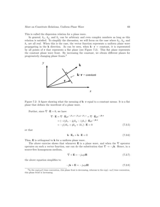
1For a comprehensive review of this topic, one may read the lecture notes [38].](https://image.slidesharecdn.com/emftall20191204-240115133321-d13ecad1/85/EMFTAll2-81-320.jpg)
![68 Electromagnetic Field Theory
One can convert the above back to the time domain using phasor technique, or by using that
Ex(z, t) = e[Ex(z, ω)ejωt
], yielding
Ex(z, t) = |E0+| cos(ωt − k0z + α+) + |E0−| cos(ωt + k0z + α−) (7.2.8)
where we have assumed that
E0± = |E0±|ejα±
(7.2.9)
The physical picture of the above expressions can be appreciated by rewriting
cos(ωt ∓ k0z + α±) = cos
ω
c0
(c0t ∓ z) + α±
(7.2.10)
where we have used the fact that k0 = ω
c0
. One can see that the first term on the right-hand
side of (7.2.8) is a sinusoidal plane wave traveling to the right, while the second term is a
sinusoidal plane wave traveling to the left, with velocity c0. The above plane wave is uniform
and a constant in the xy plane and propagating in the z direction. Hence, it is also called a
uniform plane wave in 1D.
Moreover, for a fixed t or at t = 0, the sinusoidal functions are proportional to cos(∓k0z +
α±). This is a periodic function in z with period 2π/k0 which is the wavelength λ0, or that
k0 =
2π
λ0
=
ω
c0
=
2πf
c0
(7.2.11)
One can see that because c0 is a humongous number, λ0 can be very large. You can plug in
the frequency of your local AM station to see how big λ0 is.
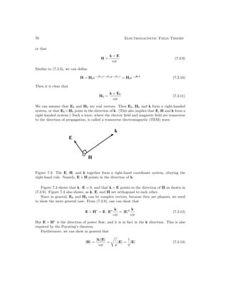
7.3 Uniform Plane Waves in 3D
By repeating the previous derivation for a homogeneous lossless medium, the vector Helmholtz
equation for a source-free medium is given by [38]
∇ × ∇ × E − ω2
µεE = 0 (7.3.1)
By the same derivation as before for the free-space case, one has
∇2
E + ω2
µεE = 0 (7.3.2)
if ∇ · E = 0.
The general solution to (7.3.2) is hence
E = E0e−jkxx−jkyy−jkzz
= E0e−jk·r
(7.3.3)
where k = x̂kx + ŷky + ẑkz, r = x̂x + ŷy + ẑz and E0 is a constant vector. And upon
substituting (7.3.3) into (7.3.2), it is seen that
k2
x + k2
y + k2
z = ω2
µε (7.3.4)](https://image.slidesharecdn.com/emftall20191204-240115133321-d13ecad1/85/EMFTAll2-82-320.jpg)

![Lossy Media, Lorentz Force Law, Drude-Lorentz-Sommerfeld Model 75
current, or that σ ωε. This happens for radio wave propagating in the saline solution of
the ocean, the Earth, or wave propagating in highly conductive metal, like your induction
cooker.
When the conductivity is low, namely, when the displacement current is larger than the
conduction current, then σ
ωε 1, we have
k = ω
r
µ
ε − j
σ
ω
= ω
s
µε
1 −
jσ
ωε
≈ ω
√
µε
1 − j
1
2
σ
ωε
= k0
− jk00
(8.1.13)
The term σ
ωε is called the loss tangent of a lossy medium.
In general, in a lossy medium ε = ε0
− jε00
, ε00
/ε0
is called the loss tangent of the medium.
It is to be noted that in the optics and physics community, e−iωt
time convention is preferred.
In that case, we need to do the switch j → −i, and a loss medium is denoted by ε = ε0
+ iε00
.
8.2 Lorentz Force Law
The Lorentz force law is the generalization of the Coulomb’s law for forces between two
charges. Lorentz force law includes the presence of a magnetic field. The Lorentz force law
is given by
F = qE + qv × B (8.2.1)
The first term electric force similar to the statement of Coulomb’s law, while the second term
is the magnetic force called the v × B force. This law can be also written in terms of the
force density f which is the force on the charge density, instead of force on a single charge.
By so doing, we arrive at
f = %E + %v × B = %E + J × B (8.2.2)
where % is the charge density, and one can identified the current J = %v.
Lorentz force law can also be derived from the integral form of Faraday’s law, if one
assumes that the law is applied to a moving loop intercepting a magnetic flux [60]. In other
words, Lorentz force law and Faraday’s law are commensurate with each other.
8.3 Drude-Lorentz-Sommerfeld Model
In the previous lecture, we have seen how loss can be introduced by having a conduction
current flowing in a medium. Now that we have learnt the versatility of the frequency domain
method, other loss mechanism can be easily introduced with the frequency-domain method.
First, let us look at the simple constitutive relation where
D = ε0E + P (8.3.1)](https://image.slidesharecdn.com/emftall20191204-240115133321-d13ecad1/85/EMFTAll2-89-320.jpg)
![76 Electromagnetic Field Theory
We have a simple model where
P = ε0χ0E (8.3.2)
where χ0 is the electric susceptibility. To see how χ0(ω) can be derived, we will study the
Drude-Lorentz-Sommerfeld model. This is usually just known as the Drude model or the
Lorentz model in many textbooks although Sommerfeld also contributed to it. This model
can be unified in one equation as shall be shown.
We can first start with a simple electron driven by an electric field E in the absence of a
magnetic field B. If the electron is free to move, then the force acting on it, from the Lorentz
force law, is −eE where e is the charge of the electron. Then from Newton’s law, assuming a
one dimensional case, it follows that
me
d2
x
dt2
= −eE (8.3.3)
where the left-hand side is due to the inertial force of the mass of the electron, and the right-
hand side is the electric force acting on a charge of −e coulomb. Here, we assume that E
points in the x-direction, and we neglect the vector nature of the electric field. Writing the
above in the frequency domain for time-harmonic fields, and using phasor technique, one gets
−ω2
mex = −eE (8.3.4)
From this, we have
x =
e
ω2me
E (8.3.5)
This for instance, can happen in a plasma medium where the atoms are ionized, and the
electrons are free to roam [61]. Hence, we assume that the positive ions are more massive,
and move very little compared to the electrons when an electric field is applied.
Figure 8.1: Polarization of an atom in the presence of an electric field. Here, it is assumed
that the electron is weakly bound or unbound to the nucleus of the atom.
The dipole moment formed by the displaced electron away from the ion due to the electric
field is
p = −ex = −
e2
ω2me
E (8.3.6)](https://image.slidesharecdn.com/emftall20191204-240115133321-d13ecad1/85/EMFTAll2-90-320.jpg)
![Lossy Media, Lorentz Force Law, Drude-Lorentz-Sommerfeld Model 79
χ0 exhibits a large negative imaginary part, the hallmark of a dissipative medium, as in the
conducting medium we have previously studied.
The DLS model is a wonderful model because it can capture phenomenologically the
essence of the physics of many electromagnetic media, even though it is a purely classical
model.1
It captures the resonance behavior of an atom absorbing energy from light excitation.
When the light wave comes in at the correct frequency, it will excite electronic transition
within an atom which can be approximately modeled as a resonator with behavior similar to
that of a pendulum oscillator. This electronic resonances will be radiationally damped [33],
and the damped oscillation can be modeled by Γ 6= 0.
Moreover, the above model can also be used to model molecular vibrations. In this case,
the mass of the electron will be replaced by the mass of the atom involved. The damping of
the molecular vibration is caused by the hindered vibration of the molecule due to interaction
with other molecules [62]. The hindered rotation or vibration of water molecules when excited
by microwave is the source of heat in microwave heating.
In the case of plasma, Γ 6= 0 represents the collision frequency between the free electrons
and the ions, giving rise to loss. In the case of a conductor, Γ represents the collision frequency
between the conduction electrons in the conduction band with the lattice of the material.2
Also, if there is no restoring force, then ω0 = 0. This is true for sea of electron moving in the
conduction band of a medium. Also, for sufficiently low frequency, the inertial force can be
ignored. Thus, from (8.3.16)
χ0 ≈ −j
ωp
2
ωΓ
(8.3.18)
and
ε = ε0(1 + χ0) = ε0
1 − j
ωp
2
ωΓ
(8.3.19)
We recall that for a conductive medium, we define a complex permittivity to be
ε = ε0
1 − j
σ
ωε0
(8.3.20)
Comparing (8.3.19) and (8.3.20), we see that
σ = ε0
ωp
2
Γ
(8.3.21)
The above formula for conductivity can be arrived at using collision frequency argument as
is done in some textbooks [65].
Because the DLS is so powerful, it can be used to explain a wide range of phenomena
from very low frequency to optical frequency.
1What we mean here is that only Newton’s law has been used, and no quantum theory as yet.
2It is to be noted that electron has a different effective mass in a crystal lattice [63, 64], and hence, the
electron mass has to be changed accordingly in the DLS model.](https://image.slidesharecdn.com/emftall20191204-240115133321-d13ecad1/85/EMFTAll2-93-320.jpg)
![Lossy Media, Lorentz Force Law, Drude-Lorentz-Sommerfeld Model 81
8.3.2 Plasmonic Nanoparticles
When a plasmonic nanoparticle made of gold is excited by light, its response is given by (see
homework assignment)
ΦR = E0
a3
cos θ
r2
εs − ε0
εs + 2ε0
(8.3.25)
In a plasma, εs can be negative, and thus, at certain frequency, if εs = −2ε0, then ΦR → ∞.
Therefore, when light interacts with such a particle, it can sparkle brighter than normal. This
reminds us of the saying “All that glitters is not gold!” even though this saying has a different
intended meaning.
Ancient Romans apparently knew about the potent effect of using gold and silver nanopar-
ticles to enhance the reflection of light. These nanoparticles were impregnated in the glass
or lacquer ware. By impregnating these particles in different media, the color of light will
sparkle at different frequencies, and hence, the color of the glass emulsion can be changed
(see website [66]).
Figure 8.3: Ancient Roman goblets whose laquer coating glisten better due to the presence
of gold nanoparticles (courtesy of Smithsonian.com).](https://image.slidesharecdn.com/emftall20191204-240115133321-d13ecad1/85/EMFTAll2-95-320.jpg)

![Lecture 9
Waves in Gyrotropic Media,
Polarization
9.1 Gyrotropic Media
This section presents deriving the permittivity tensor of a gyrotropic medium in the ionsphere.
Our ionosphere is always biased by a static magnetic field due to the Earth’s magnetic field
[67]. But in this derivation, one assumes that the ionosphere has a static magnetic field
polarized in the z direction, namely that B = ẑB0. Now, the equation of motion from the
Lorentz force law for an electron with q = −e, in accordance with Newton’s law, becomes
me
dv
dt
= −e(E + v × B) (9.1.1)
Next, let us assume that the electric field is polarized in the xy plane. The derivative of v
is the acceleration of the electron, and also, v = dr/dt. And in the frequency domain, the
above equation becomes
meω2
x = e(Ex + jωB0y) (9.1.2)
meω2
y = e(Ey − jωB0x) (9.1.3)
The above equations cannot be solved easily for x and y in terms of the electric field
because they correspond to a two-by-two matrix system with cross coupling between the
unknowns x and y. But they can be simplified as follows: We can multiply (9.1.3) by ±j and
add it to (9.1.2) to get two decoupled equations [68]:
meω2
(x + jy) = e[(Ex + jEy) + ωB0(x + jy)] (9.1.4)
meω2
(x − jy) = e[(Ex − jEy) − ωB0(x − jy)] (9.1.5)
Defining new variables such that
s± = x ± jy (9.1.6)
E± = Ex ± jEy (9.1.7)
83](https://image.slidesharecdn.com/emftall20191204-240115133321-d13ecad1/85/EMFTAll2-97-320.jpg)
![84 Electromagnetic Field Theory
then (9.1.4) and (9.1.5) become
meω2
s± = e(E± ± ωB0s±) (9.1.8)
Thus, solving the above yields
s± =
e
meω2 ∓ eB0ω
E± = C±E± (9.1.9)
where
C± =
e
meω2 ∓ eB0ω
(9.1.10)
By this manipulation, the above equations (9.1.2) and (9.1.3) transform to new equations
where there is no cross coupling between s± and E±. The mathematical parlance for this is
the diagnolization of a matrix equation [69]. Thus, the new equation can be solved easily.
Next, one can define Px = −Nex, Py = −Ney, and that P± = Px ± jPy = −Nes±. Then
it can be shown that
P± = ε0χ±E± (9.1.11)
The expression for χ± can be derived, and they are given as
χ± = −
NeC±
ε0
= −
Ne
ε0
e
meω2 ∓ eBoω
= −
ωp
2
ω2 ∓ Ωω
(9.1.12)
where Ω and ωp are the cyclotron frequency1
and plasma frequency, respectively.
Ω =
eB0
me
, ωp
2
=
Ne2
meε0
(9.1.13)
At the cyclotron frequency, a solution exists to the equation of motion (9.1.1) without a
forcing term, which in this case is the electric field E = 0. Thus, at this frequency, the
solution blows up if the forcing term, E± is not zero. This is like what happens to an LC
tank circuit at resonance whose current or voltage tends to infinity when the forcing term,
like the voltage or current is nonzero.
Now, one can rewrite (9.1.11) in terms of the original variables Px, Py, Ex, Ey, or
Px =
P+ + P−
2
=
ε0
2
(χ+E+ + χ−E−) =
ε0
2
[χ+(Ex + jEy) + χ−(Ex − jEy)]
=
ε0
2
[(χ+ + χ−)Ex + j(χ+ − χ−)Ey] (9.1.14)
Py =
P+ − P−
2j
=
ε0
2j
(χ+E+ − χ−E−) =
ε0
2j
[χ+(Ex + jEy) − χ−(Ex − jEy)]
=
ε0
2j
[(χ+ − χ−)Ex + j(χ+ + χ−)Ey] (9.1.15)
1This is also called the gyrofrequency.](https://image.slidesharecdn.com/emftall20191204-240115133321-d13ecad1/85/EMFTAll2-98-320.jpg)
![Waves in Gyrotropic Media, Polarization 85
The above relationship can be expressed using a tensor where
P = ε0χ
χ
χ · E (9.1.16)
where P = [Px, Py], and E = [Ex, Ey]. From the above, χ is of the form
χ =
1
2
(χ+ + χ−) j(χ+ − χ−)
−j(χ+ − χ−) (χ+ + χ−)
=
−
ωp
2
ω2−Ω2 −j
ωp
2
Ω
ω(ω2−Ω2)
j
ωp
2
Ω
ω(ω2−Ω2) −
ωp
2
ω2−Ω2
!
(9.1.17)
Notice that in the above, when the B field is turned off or Ω = 0, the above resembles the
solution of a collisionless, cold plasma.
For the electric field in the z direction, it will drive a motion of the electron to be in the
z direction. In this case, v × B term is zero, and the electron motion is unaffected by the
magnetic field as can be seen from the Lorentz force law or (9.1.1). Hence, it behaves like a
simple collisionless plasma without a biasing magnetic field. Consequently, the above can be
generalized to 3D to give
χ =
χ0 jχ1 0
−jχ1 χ0 0
0 0 χp
(9.1.18)
where χp = −ω2
p/ω2
.
Using the fact that D = ε0E + P = ε0(I + χ) · E = ε · E, the above implies that
ε = ε0
1 + χ0 jχ1 0
−jχ1 1 + χ0 0
0 0 1 + χp
(9.1.19)
Please notice that the above tensor is a hermitian tensor. We shall learn later that this is the
hallmark of a lossless medium.
Another characteristic of a gyrotropic medium is that a linearly polarized wave will rotate
when passing through it. This is the Faraday rotation effect [68], which we shall learn later.
This phenomenon poses a severe problem to Earth-to-satellite communication, using linearly
polarized wave as it requires the alignment of the Earth-to-satellite antennas. This can be
avoided using a rotatingly polarized wave, called a circularly polarized wave that we shall learn
in the next section. Also, the ionosphere of the Earth is highly dependent on temperature, and
the effect of the Sun. The fluctuation of particles in the ionosphere gives rise to scintillation
effects that affect radio wave communication systems [70].
9.2 Wave Polarization
Studying wave polarization is very important for communication purposes [31]. A wave whose
electric field is pointing in the x direction while propagating in the z direction is a linearly
polarized (LP) wave. The same can be said of one with electric field polarized in the y
direction. It turns out that a linearly polarized wave suffers from Faraday rotation when](https://image.slidesharecdn.com/emftall20191204-240115133321-d13ecad1/85/EMFTAll2-99-320.jpg)
![86 Electromagnetic Field Theory
it propagates through the ionosphere. For instance, an x polarized wave can become a y
polarized due to Faraday rotation. So its polarization becomes ambiguous: to overcome this,
Earth to satellite communication is done with circularly polarized (CP) waves [71]. So even
if the electric field vector is rotated by Faraday’s rotation, it remains to be a CP wave. We
will study these polarized waves next.
We can write a general uniform plane wave propagating in the z direction as
E = x̂Ex(z, t) + ŷEy(z, t) (9.2.1)
Clearly, ∇ · E = 0, and Ex(z, t) and Ey(z, t) are solutions to the one-dimensional wave
equation. For a time harmonic field, the two components may not be in phase, and we have
in general
Ex(z, t) = E1 cos(ωt − βz) (9.2.2)
Ey(z, t) = E2 cos(ωt − βz + α) (9.2.3)
where α denotes the phase difference between these two wave components. We shall study
how the linear superposition of these two components behaves for different α’s. First, we set
z = 0 to observe this field. Then
E = x̂E1 cos(ωt) + ŷE2 cos(ωt + α) (9.2.4)
For α = π
2
Ex = E1 cos(ωt), Ey = Ez cos(ωt + π/2) (9.2.5)
Next, we evaluate the above for different ωt’s
ωt = 0, Ex = E1, Ey = 0 (9.2.6)
ωt = π/4, Ex = E1/
√
2, Ey = −E2/
√
2 (9.2.7)
ωt = π/2, Ex = 0, Ey = −E2 (9.2.8)
ωt = 3π/4, Ex = −E1/
√
2, Ey = −E2/
√
2 (9.2.9)
ωt = π, Ex = −E1, Ey = 0 (9.2.10)
The tip of the vector field E traces out an ellipse as show in Figure 9.1. With the thumb
pointing in the z direction, and the wave rotating in the direction of the fingers, such a wave
is called left-hand elliptically polarized (LHEP) wave.](https://image.slidesharecdn.com/emftall20191204-240115133321-d13ecad1/85/EMFTAll2-100-320.jpg)
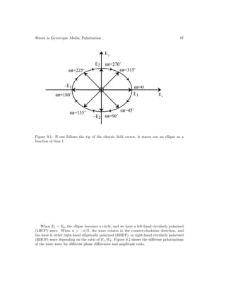
![88 Electromagnetic Field Theory
Figure 9.2: Due to different phase difference between the Ex and Ey components of the
field, and their relative amplitudes E2/E1, different polarizations will ensure. The arrow
indicates the direction of rotation of the field vector. In this figure, ψ = −α in our notes, and
A = E2/E1 (Courtesy of J.A. Kong, Electromagnetic Wave Theory [31]).
Figure 9.3 shows a graphic picture of a CP wave propagating through space.](https://image.slidesharecdn.com/emftall20191204-240115133321-d13ecad1/85/EMFTAll2-102-320.jpg)
![Waves in Gyrotropic Media, Polarization 89
Figure 9.3: The rotation of the field vector of a right-hand circular polarization wave as it
propagates in the right direction [72] (Courtesy of Wikipedia).
9.2.1 Arbitrary Polarization Case and Axial Ratio
The axial ratio (AR) is an important figure of merit for designing CP antennas (antennas
that will radiate CP or circularly polarized waves). The closer is this ratio to 1, the better
the antenna design. We will discuss the general polarization and the axial ratio of a wave.
For the general case for arbitrary α, we let
Ex = E1 cos ωt, Ey = E2 cos(ωt + α) = E2(cos ωt cos α − sin ωt sin α) (9.2.11)
Then from the above, expressing Ey in terms of Ex, one gets
Ey =
E2
E1
Ex cos α − E2
1 −
Ex
E1
2
1/2
sin α (9.2.12)
Rearranging and squaring, we get
aEx
2
− bExEy + cEy
2
= 1 (9.2.13)
where
a =
1
E1
2
sin2
α
, b =
2 cos α
E1E2 sin2
α
, c =
1
E2
2
sin2
α
(9.2.14)
After letting Ex → x, and Ey → y, equation (9.2.13) is of the form,
ax2
− bxy + cy2
= 1 (9.2.15)](https://image.slidesharecdn.com/emftall20191204-240115133321-d13ecad1/85/EMFTAll2-103-320.jpg)
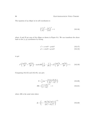
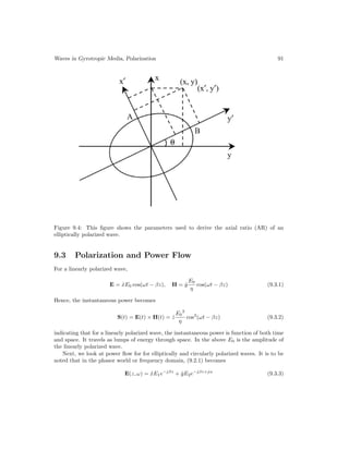
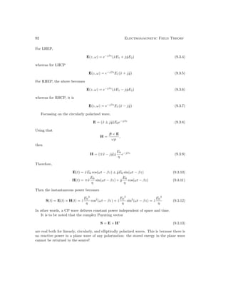
![94 Electromagnetic Field Theory
ŷ = ρ̂ sin φ + φ̂ cos φ, then a CP field is proportional to
(x̂ ± jŷ) = ρ̂e±jφ
± jφ̂e±jφ
= e±jφ
(ρ̂ ± φ̂) (10.1.1)
Therefore, the ρ̂ and φ̂ of a CP is also an azimuthal traveling wave in the φ̂ direction in
addition to being a traveling wave e−jβz
in the ẑ direction. This is obviated by writing
e−jφ
= e−jkφρφ
(10.1.2)
where kφ = 1/ρ is the azimuthal wave number, and ρφ is the arc length traversed by the
azimuthal wave. Notice that the wavenumber kφ is dependent on ρ: the larger the ρ, the
larger the azimuthal wavelength.
Thus, the wave possesses angular momentum called the spin angular momentum (SAM),
just as a traveling wave e−jβz
possesses linear angular momentum in the ẑ direction.
In optics research, the generation of cylindrical vector beam is in vogue. Figure 10.2 shows
a method to generate such a beam. A CP light passes through a radial analyzer that will only
allow the radial component of (10.1.1) to be transmitted. Then a spiral phase element (SPE)
compensates for the exp(±jφ) phase shift in the azimuthal direction. Finally, the light is a
cylindrical vector beam which is radially polarized without spin angular momentum. Such
a beam has been found to have nice focussing property, and hence, has aroused researchers’
interest in the optics community [73].
Figure 10.2: A cylindrical vector beam can be generated experimentally (courtesy of Zhan,
Q. [73]).](https://image.slidesharecdn.com/emftall20191204-240115133321-d13ecad1/85/EMFTAll2-108-320.jpg)
![Spin Angular Momentum, Complex Poynting’s Theorem, Lossless Condition, Energy Density95
10.2 Complex Poynting’s Theorem and Lossless Condi-
tions
10.2.1 Complex Poynting’s Theorem
It has been previously shown that the vector E(r, t) × H(r, t) has a dimension of watts/m2
which is that of power density. Therefore, it is associated with the direction of power flow
[31, 42]. As has been shown for time-harmonic field, a time average of this vector can be
defined as
hE(r, t) × H(r, t)i = lim
T →∞
1
T
T
0
E(r, t) × H(r, t) dt. (10.2.1)
Given the phasors of time harmonic fields E(r, t) and H(r, t), namely, E(r, ω) and H(r, ω)
respectively, we can show that
hE(r, t) × H(r, t)i =
1
2
e{E(r, ω) × H∗
(r, ω)}. (10.2.2)
Here, the vector E(r, ω) × H∗
(r, ω), as previously discussed, is also known as the complex
Poynting vector. Moreover, because of its aforementioned property, and its dimension of
power density, we will study its conservative property. To do so, we take its divergence and
use the appropriate vector identity to obtain1
∇ · (E × H∗
) = H∗
· ∇ × E − E · ∇ × H∗
. (10.2.3)
Next, using Maxwell’s equations for ∇ × E and ∇ × H∗
, namely
∇ × E = −jωB (10.2.4)
∇ × H∗
= −jωD∗
+ J∗
(10.2.5)
and the constitutive relations for anisotropic media that
B = µ · H, D∗
= ε∗
· E∗
(10.2.6)
we have
∇ · (E × H∗
) = −jω H∗
· B + jω E · D∗
− E · J∗
(10.2.7)
= −jω H∗
· µ · H + jω E · ε∗
· E∗
− E · J∗
. (10.2.8)
The above is also known as the complex Poynting’s theorem. It can also be written in an
integral form using Gauss’ divergence theorem, namely,
S
dS · (E × H∗
) = −jω
V
dV (H∗
· µ · H − E · ε∗
· E∗
) −
V
dV E · J∗
. (10.2.9)
where S is the surface bounding the volume V .
1We will drop the argument r, ω for the phasors in our discussion next as they will be implied.](https://image.slidesharecdn.com/emftall20191204-240115133321-d13ecad1/85/EMFTAll2-109-320.jpg)
![Spin Angular Momentum, Complex Poynting’s Theorem, Lossless Condition, Energy Density97
But the above, using that =m(Z) = 1/(2j)(Z − Z∗
), is the same as
−j
V
dV [H∗
· (µ†
− µ) · H + E∗
· (ε†
− ε) · E] 0. (10.2.15)
Therefore, for a medium to be lossy, −j(µ†
− µ) and −j(ε†
− ε) must be hermitian, positive
definite matrices, to ensure the inequality in (10.2.15). Similarly, for an active medium,
−j(µ†
− µ) and −j(ε†
− ε) must be hermitian, negative definite matrices.
For a lossy medium which is conductive, we may define J = σ · E where σ is a general
conductivity tensor. In this case, equation (10.2.9), after combining the last two terms, may
be written as
S
dS · (E × H∗
) = −jω
V
dV
H∗
· µ · H − E ·
ε∗
+
jσ∗
ω
· E∗
(10.2.16)
= −jω
dV [H∗
· µ · H − E · ε̃
∗
· E∗
], (10.2.17)
where ε̃ = ε − jσ
ω which, in general, is the complex permittivity tensor. In this manner,
(10.2.17) has the same structure as the source-free Poynting’s theorem. Notice here that the
complex permittivity tensor ε̃ is clearly non-hermitian corresponding to a lossy medium.
For a lossless medium without the source term, by taking the imaginary part of (10.2.9),
we arrive at
=m
S
dS · (E × H∗
) = −ω
V
dV (H∗
· µ · H − E · ε∗
· E∗
), (10.2.18)
The left-hand side of the above is the reactive power coming out of the volume V , and hence,
the right-hand side can be interpreted as reactive power as well. It is to be noted that
H∗
· µ · H and E · ε∗
· E∗
are not to be interpreted as stored energy density when the medium
is dispersive. The correct expressions for stored energy density will be derived in the next
section.
But, the quantity H∗
· µ · H for lossless, dispersionless media is associated with the time-
averaged energy density stored in the magnetic field, while the quantity E · ε∗
· E∗
for lossless
dispersionless media is associated with the time-averaged energy density stored in the electric
field. Then, for lossless, dispersionless, source-free media, then the right-hand side of the
above can be interpreted as stored energy density. Hence, the reactive power is proportional
to the time rate of change of the difference of the time-averaged energy stored in the magnetic
field and the electric field.
10.3 Energy Density in Dispersive Media
A dispersive medium alters our concept of what energy density is.3
To this end, we assume
that the field has complex ω dependence in ejωt
, where ω = ω0
− jω00
, rather than real ω de-
3The derivation here is inspired by H.A. Haus, Electromagnetic Noise and Quantum Optical Measurements
[74]. Generalization to anisotropic media is given by W.C. Chew, Lectures on Theory of Microwave and Optical
Waveguides [75].](https://image.slidesharecdn.com/emftall20191204-240115133321-d13ecad1/85/EMFTAll2-111-320.jpg)
![98 Electromagnetic Field Theory
pendence. We take the divergence of the complex power for fields with such time dependence,
and let ejωt
be attached to the field. So E(t) and H(t) are complex field but not exactly like
phasors since they are not truly time harmonic. In other words, we let
E(r, t) = E
e
(r, ω)ejωt
, H(r, t) = H
e
(r, ω)ejωt
(10.3.1)
The above, just like phasors, can be made to satisfy Maxwell’s equations where the time
derivative becomes jω. We can study the quantity E(r, t) × H∗
(r, t) which has the unit of
power density. In the real ω case, their time dependence will exactly cancel each other and
this quantity becomes complex power again, but not in the complex ω case. Hence,
∇ · [E(t) × H∗
(t)] = H∗
(t) · ∇ × E(t) − E(t) · ∇ × H∗
(t)
= −H∗
(t) · jωµH(t) + E(t) · jω∗
ε∗
E∗
(10.3.2)
where Maxwell’s equations have been used to substitute for ∇ × E(t) and ∇ × H∗
(t). The
space dependence of the field is implied, and we assure a source-free medium so that J = 0.
If E(t) ∼ ejωt
, then, due to ω being complex, now H∗
(t) ∼ e−jω∗
t
, and the term like
E(t) × H∗
(t) is not truly time independent,
E(t) × H∗
(t) ∼ ej(ω−ω∗
)t
= e2ω00
t
(10.3.3)
And each of the term above will have similar time dependence. Writing (10.3.2) more explic-
itly, by letting ω = ω0
− jω00
, we have
∇ · [E(t) × H∗
(t)] = −j(ω0
− jω00
)µ(ω)|H(t)|2
+ j(ω0
+ jω00
)ε∗
(ω)|E(t)|2
(10.3.4)
Assuming that ω00
ω0
, or that the field is quasi-time-harmonic, we can let, after using
Taylor series approximation, that
µ(ω0
− jω00
) ∼
= µ(ω0
) − jω00 ∂µ(ω0
)
∂ω0
, ε(ω0
− jω00
) ∼
= ε(ω0
) − jω00 ∂ε(ω0
)
∂ω0
(10.3.5)
Using (10.3.5) in (10.3.4), and collecting terms of the same order, and ignoring (ω00
)2
terms,
gives
∇ · [E(t) × H∗
(t)] ∼
= − jω0
µ(ω0
)|H(t)|2
+ jω0
ε∗
(ω0
)|E(t)|2
− ω00
µ(ω0
)|H(t)|2
− ω0
ω00 ∂µ
∂ω0
|H(t)|2
− ω00
ε∗
(ω0
)|E(t)|2
− ω0
ω00 ∂ε∗
∂ω0
|E(t)|2
(10.3.6)
The above can be rewritten as
∇ · [E(t) × H∗
(t)] ∼
= −jω0
µ(ω0
)|H(t)|2
− ε∗
(ω0
)|E(t)|2
− ω00
∂ω0
µ(ω0
)
∂ω0
|H(t)|2
+
∂ω0
ε∗
(ω0
)
∂ω0
|E(t)|2
(10.3.7)](https://image.slidesharecdn.com/emftall20191204-240115133321-d13ecad1/85/EMFTAll2-112-320.jpg)
![Spin Angular Momentum, Complex Poynting’s Theorem, Lossless Condition, Energy Density99
The above approximation is extremely good when ω00
ω0
. For a lossless medium, ε(ω0
) and
µ(ω0
) are purely real, and the first term of the right-hand side is purely imaginary while the
second term is purely real. In the limit when ω00
→ 0, when we take half the imaginary part
of the above equation, we have
∇ ·
1
2
=m [E × H∗
] = −ω0
1
2
µ|H|2
−
1
2
ε|E|2
(10.3.8)
which has the physical interpretation of reactive power as has been previously discussed.
When we take half the real part of (10.3.7), we obtain
∇ ·
1
2
e[E × H∗
] = −
ω00
2
∂ω0
µ
∂ω0
|H|2
+
∂ω0
ε
∂ω0
|E|2
(10.3.9)
Since the right-hand side has time dependence of e2ω00
t
, it can be written as
∇ ·
1
2
e[E × H∗
] = −
∂
∂t
1
4
∂ω0
µ
∂ω0
|H|2
+
∂ω0
ε
∂ω0
|E|2
= −
∂
∂t
hWT i (10.3.10)
Therefore, the time-average stored energy density can be identified as
hWT i =
1
4
∂ω0
µ
∂ω0
|H|2
+
∂ω0
ε
∂ω0
|E|2
(10.3.11)
For a non-dispersive medium, the above reduces to
hWT i =
1
4
µ|H|2
+ ε|E|2
(10.3.12)
which is what we have derived before. In the above analysis, we have used a quasi-time-
harmonic signal with exp(jωt) dependence. In the limit when ω00
→ 0, this signal reverts
back to a time-harmonic signal, and to our usual interpretation of complex power. However,
by assuming the frequency ω to have a small imaginary part ω00
, it forces the stored energy
to grow very slightly, and hence, power has to be supplied to maintain the growth of this
stored energy. By so doing, it allows us to identify the expression for energy density for a
dispersive medium. These expressions for energy density were not discovered until 1960 by
Brillouin [76], as energy density times group velocity should be power flow. More discussion
on this topic can be found in Jackson [42].
It is to be noted that if the same analysis is used to study the energy storage in a capacitor
or an inductor, the energy storage formulas have to be accordingly modified if the capacitor
or inductor is frequency dependent.](https://image.slidesharecdn.com/emftall20191204-240115133321-d13ecad1/85/EMFTAll2-113-320.jpg)

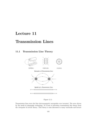
![102 Electromagnetic Field Theory
notes. Transmission lines are so important in modern day electromagnetic engineering, that
most engineering electromagnetics textbooks would be incomplete without introducing the
topic [29,31,38,47,48,59,71,75,77,78].
Circuit theory is robust and is not sensitive to the detail shapes of the components in-
volved such as capacitors or inductors. Moreover, many transmission line problems cannot
be analyzed with the full form of Maxwell’s equations,1
but approximate solutions can be
obtained using circuit theory in the long-wavelength limit. We shall show that circuit theory
is an approximation of electromagnetic field theory when the wavelength is very long: the
longer the wavelength, the better is the approximation [47].
Examples of transmission lines are shown in Figure 11.1. The symbol for a transmission
line is usually represented by two pieces of parallel wires, but in practice, these wires need
not be parallel.
Figure 11.2: Courtesy of slides by A. Wadhwa, A.L. Dal, N. Malhotra [79].
Circuit theory also explains why waveguides can be made sloppily when wavelength is long
or the frequency low. For instance, in the long-wavelength limit, we can make twisted-pair
waveguides with abandon, and they still work well (see Figure 11.2). Hence, we shall first
explain the propagation of electromagnetic signal on a transmission line using circuit analysis.
11.1.1 Time-Domain Analysis
We will start with performing the time-domain analysis of a simple, infinitely long trans-
mission line. Remember that two pieces of metal can accumulate attractive charges between
them, giving rise to capacitive coupling, electric field, and hence stored energy in the electric
field. Moreover, a piece of wire carrying a current generates a magnetic field, and hence,
yielding stored energy in the magnetic field. These stored energies are the sources of the
capacitive and inductive effects. But these capacitive and inductive effects are distributed
over the spatial dimension of the transmission line. Therefore, it is helpful to think of the
two pieces of metal as consisting of small segments of metal concatenated together. Each of
these segments will have a small inductance, as well as a small capacitive coupling between
them. Hence, we can model two pieces of metal with a distributed lumped element model as
shown in Figure 11.3. For simplicity, we assume the other conductor to be a ground plane,
so that it need not be approximated with lumped elements.
1Usually called full-wave analysis.](https://image.slidesharecdn.com/emftall20191204-240115133321-d13ecad1/85/EMFTAll2-116-320.jpg)
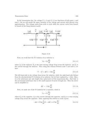
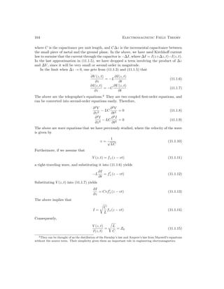
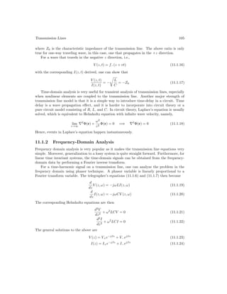
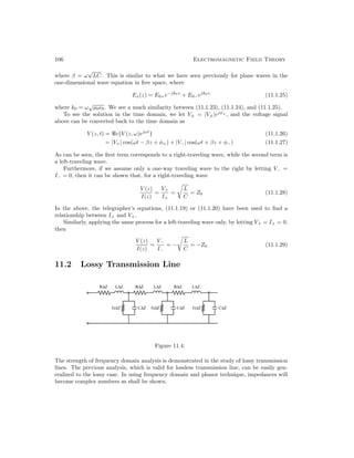
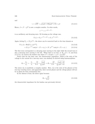
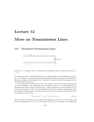
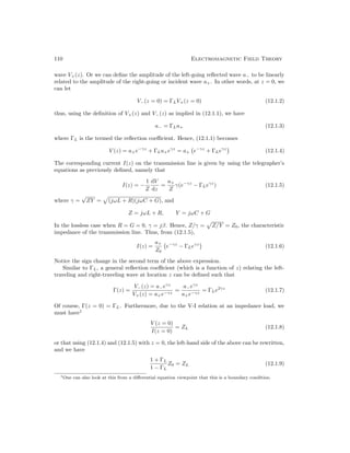
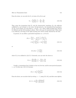
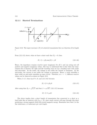
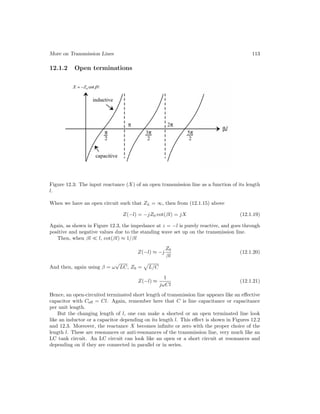
![114 Electromagnetic Field Theory
12.2 Smith Chart
In general, from (12.1.14) and (12.1.15), a length of transmission line can transform a load ZL
to a range of possible complex values Z(−l). To understand this range of values better, we
can use the Smith chart (invented by P.H. Smith 1939 before the advent of the computer) [80].
The Smith chart is essentially a graphical calculator for solving transmission line problems.
Equation (12.1.13) indicates that there is a unique map between the normalized impedance
Z(z)/Z0 and reflection coefficient Γ(z). In the normalized impedance form where Zn = Z/Z0,
from (12.1.11) and (12.1.13)
Γ =
Zn − 1
Zn + 1
, Zn =
1 + Γ
1 − Γ
(12.2.1)
Equations in (12.2.1) are related to a bilinear transform in complex variables [81]. It is a kind
of conformal map that maps circles to circles. Such a map is shown in Figure 12.4, where lines
on the right-half of the complex Zn plane are mapped to the circles on the complex Γ plane.
Since straight lines on the complex Zn plane are circles with infinite radii, they are mapped
to circles on the complex Γ plane. The Smith chart allows one to obtain the corresponding Γ
given Zn and vice versa as indicated in (12.2.1), but using a graphical calculator.
Notice that the imaginary axis on the complex Zn plane maps to the circle of unit radius on
the complex Γ plane. All points on the right-half plane are mapped to within the unit circle.
The reason being that the right-half plane of the complex Zn plane corresponds to passive
impedances that will absorb energy. Hence, such an impedance load will have reflection
coefficient with amplitude less than one, which are points within the unit circle.
On the other hand, the left-half of the complex Zn plane corresponds to impedances with
negative resistances. These will be active elements that can generate energy, and hence,
yielding |Γ| 1, and will be outside the unit circle on the complex Γ plane.
Another point to note is that points at infinity on the complex Zn plane map to the point
at Γ = 1 on the complex Γ plane, while the point zero on the complex Zn plane maps to
Γ = −1 on the complex Γ plane. These are the reflection coefficients of an open-circuit load
and a short-circuit load, respectively. For a matched load, Zn = 1, and it maps to the zero
point on the complex Γ plane implying no reflection.](https://image.slidesharecdn.com/emftall20191204-240115133321-d13ecad1/85/EMFTAll2-128-320.jpg)
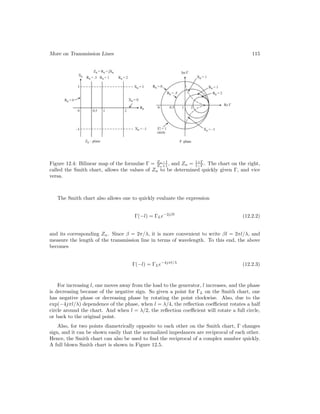
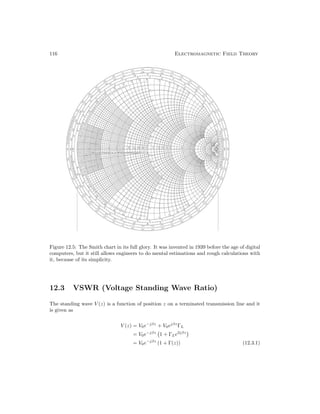
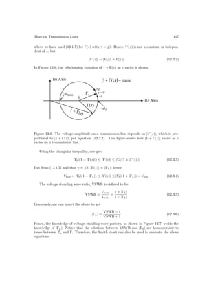
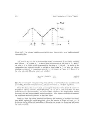
![More on Transmission Lines 119
Figure 12.8: A slotted-line equipment which consists of a coaxial waveguide with a slot
opening at the top to allow the measurement of the field strength and hence, the voltage
standing wave pattern in the waveguide (courtesy of Microwave101.com).
A typical experimental setup for a slotted line measurement is shown in Figure 12.9. A
generator source, with low frequency modulation, feeds microwave energy into the coaxial
waveguide. The isolator, allowing only the unidirectional propagation of microwave energy,
protects the generator. The attenuator protects the slotted line equipment. The wavemeter
is an adjustable resonant cavity. When the wavemeter is tuned to the frequency of the
microwave, it siphons off some energy from the source, giving rise to a dip in the signal of the
SWR meter (a short for voltage-standing-wave-ratio meter). Hence, the wavemeter measures
the frequency of the microwave.
The slotted line probe is usually connected to a square law detector that converts the
microwave signal to a low-frequency signal. In this manner, the amplitude of the voltage
in the slotted line can be measured with some low-frequency equipment, such as the SWR
meter. Low-frequency equipment is a lot cheaper to make and maintain. That is also the
reason why the source is modulated with a low-frequency signal. At low frequencies, circuit
theory prevails, engineering and design are a lot simpler.
The above describes how the impedance of the device-under-test (DUT) can be measured
at microwave frequencies. Nowadays, automated network analyzers make these measurements
a lot simpler in a microwave laboratory. More resource on microwave measurements can be
found on the web, such as in [82].
Notice that the above is based on the interference of the two traveling wave on a ter-
minated transmission line. Such interference experiments are increasingly difficult in optical
frequencies because of the much shorter wavelengths. Hence, many experiments are easier to
perform at microwave frequencies rather than at optical frequencies.
Many technologies are first developed at microwave frequency, and later developed at
optical frequency. Examples are phase imaging, optical coherence tomography, and beam
steering with phase array sources. Another example is that quantum information and quan-
tum computing can be done at optical frequency, but the recent trend is to use artificial atoms
working at microwave frequencies. Engineering with longer wavelength and larger component
is easier; and hence, microwave engineering.
Another new frontier in the electromagnetic spectrum is in the terahertz range. Due to](https://image.slidesharecdn.com/emftall20191204-240115133321-d13ecad1/85/EMFTAll2-133-320.jpg)
![120 Electromagnetic Field Theory
the dearth of sources in the terahertz range, and the added difficulty in having to engineer
smaller components, this is an exciting and a largely untapped frontier in electromagnetic
technology.
Figure 12.9: An experimental setup for a slotted line measurement (courtesy of Pozar and
Knapp, U. Mass [83]).](https://image.slidesharecdn.com/emftall20191204-240115133321-d13ecad1/85/EMFTAll2-134-320.jpg)
![Lecture 13
Multi-Junction Transmission
Lines, Duality Principle
13.1 Multi-Junction Transmission Lines
By concatenating sections of transmission lines of different characteristic impedances, a large
variety of devices such as resonators, filters, radiators, and matching networks can be formed.
We will start with a single junction transmission line first. A good reference for such problem
is the book by Collin [84], but much of the treatment here is not found in any textbooks.
13.1.1 Single-Junction Transmission Lines
Consider two transmission line connected at a single junction as shown in Figure 13.1. For
simplicity, we assume that the transmission line to the right is infinitely long so that there is no
reflected wave. And that the two transmission lines have different characteristic impedances,
Z01 and Z02.
121](https://image.slidesharecdn.com/emftall20191204-240115133321-d13ecad1/85/EMFTAll2-135-320.jpg)
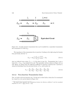
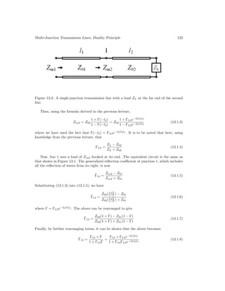
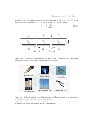
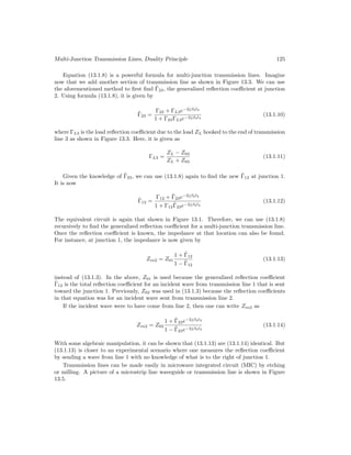

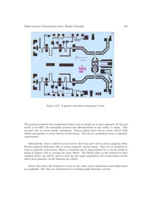
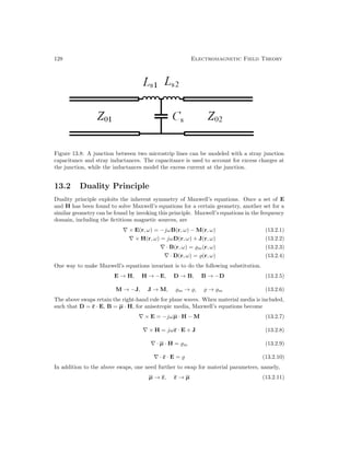
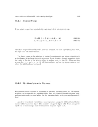
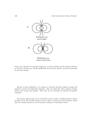
![Multi-Junction Transmission Lines, Duality Principle 131
Figure 13.10: A toroidal antenna used to drive an electric current through a conducting cylin-
der of a dipole. One can think of them as the primary and secondary turns of a transformer
(courtesy of Q. S. Liu [85]).](https://image.slidesharecdn.com/emftall20191204-240115133321-d13ecad1/85/EMFTAll2-145-320.jpg)

![Lecture 14
Reflection and Transmission,
Interesting Physical Phenomena
Much of the contents of this lecture can be found in Kong, and also the ECE 350X lecture
notes. They can be found in many textbooks, even though the notations can be slightly
different [29,31,38,47,48,59,71,75,77,78].
14.1 Reflection and Transmission—Single Interface Case
We will derive the reflection coefficients for the single interface case. These reflection co-
efficients are also called the Fresnel reflection coefficients because they were first derived by
Austin-Jean Fresnel (1788-1827). Note that he lived before the completion of Maxwell’s equa-
tions in 1865. But when Fresnel derived the reflection coefficients in 1823, they were based
on the elastic theory of light; and hence, the formulas are not exactly the same as what we
are going to derive (see Born and Wolf, Principles of Optics, p. 40 [52]).
The single-interface reflection and transmission problem is homomorphic to the transmis-
sion line problem, albeit with complicated mathematics, as we have to keep track of the 3D
polarizations of the electromagnetic fields in this case. We shall learn later that the mathe-
matical homomorphism can be used to exploit the simplicity of transmission line theory in
seeking the solutions to the multiple interface problems.
133](https://image.slidesharecdn.com/emftall20191204-240115133321-d13ecad1/85/EMFTAll2-147-320.jpg)
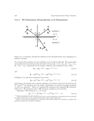
![Reflection and Transmission, Interesting Physical Phenomena 135
In order for the above to be valid for all x, it is necessary that βix = βrx = βtx, which is also
known as the phase matching condition.3
From the above, by letting βix = βrx = β1 sin θi =
β1 sin θr, we obtain that θr = θi or that the law of reflection that the angle of reflection is
equal to the angle of incidence. By letting βtx = β2 sin θt = βix = β1 sin θi, we obtain Snell’s
law that β1 sin θi = β2 sin θt. (This law of refraction that was also known in the Islamic world
in the 900 AD. [86]). Now, canceling common terms on both sides of the equation (14.1.4),
the above simplifies to
1 + RT E
= TT E
(14.1.5)
To impose n̂ × H continuous, one needs to find the H field using ∇ × E = −jωµH, or
that H = −jβ × E/(−jωµ) = β × E/(ωµ). By so doing
Hi =
βi × Ei
ωµ1
=
βi × ŷ
ωµ1
E0e−jβi·r
=
ẑβix − x̂βiz
ωµ1
E0e−jβi·r
(14.1.6)
Hr =
βr × Er
ωµ1
=
βr × ŷ
ωµ1
RT E
E0e−jβr·r
=
ẑβrx + x̂βrz
ωµ2
RT E
E0e−jβr·r
(14.1.7)
Ht =
βt × Et
ωµ2
=
βt × ŷ
ωµ2
TT E
E0e−jβt·r
=
ẑβtx − x̂βtz
ωµ2
TT E
E0e−jβt·r
(14.1.8)
Imposing n̂ × H continuous or Hx continuous at z = 0, we have
βiz
ωµ1
E0e−jβixx
−
βrz
ωµ1
RT E
E0e−jβrxx
=
βtz
ωµ2
TT E
E0e−jβtxx
(14.1.9)
As mentioned before, the phase-matching condition requires that βix = βrx = βtx. The
dispersion relation for plane waves requires that
β2
ix + β2
iz = β2
rx + β2
rz = ω2
µ1ε1 = β2
1 (14.1.10)
β2
tx + β2
tz = ω2
µ2ε2 = β2
2 (14.1.11)
Since βix = βrx = βtx = βx, the above implies that βiz = βrz = β1z. Moreover, βtz = β2z 6=
β1z usually since β1 6= β2. Then (14.1.9) simplifies to
β1z
µ1
(1 − RT E
) =
β2z
µ2
TT E
(14.1.12)
where β1z =
p
β2
1 − β2
x, and β2z =
p
β2
2 − β2
x.
Solving (14.1.5) and (14.1.12) yields
RT E
=
β1z
µ1
−
β2z
µ2
,
β1z
µ1
+
β2z
µ2
(14.1.13)
TT E
= 2
β1z
µ1
,
β1z
µ1
+
β2z
µ2
(14.1.14)
3The phase-matching condition can also be proved by taking the Fourier transform of the equation with
respect to x. Among the physics community, this is also known as momentum matching, as the wavenumber
of a wave is related to the momentum of the particle.](https://image.slidesharecdn.com/emftall20191204-240115133321-d13ecad1/85/EMFTAll2-149-320.jpg)
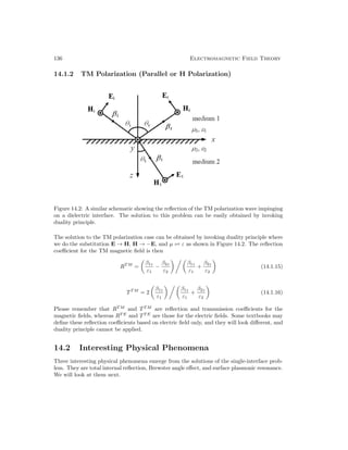
![Reflection and Transmission, Interesting Physical Phenomena 137
14.2.1 Total Internal Reflection
Total internal reflection comes about because of phase matching (also called momentum
matching). This phase-matching condition can be illustrated using β-surfaces (same as k-
surfaces in some literature), as shown in Figure 14.3. It turns out that because of phase
matching, for certain interfaces, β2z becomes pure imaginary.
Figure 14.3: Courtesy of J.A. Kong, Electromagnetic Wave Theory [31]. Here, k is synony-
mous with β. Also, the x axis is equivalent to the z axis in the previous figure.](https://image.slidesharecdn.com/emftall20191204-240115133321-d13ecad1/85/EMFTAll2-151-320.jpg)
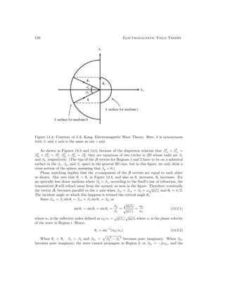
![Reflection and Transmission, Interesting Physical Phenomena 139
wave becomes evanescent. The reflection coefficient (14.1.13) becomes of the form
RT E
= (A − jB)/(A + jB) (14.2.3)
It is clear that |RT E
| = 1 and that RT E
= ejθT E
. Therefore, a total internally reflected wave
suffers a phase shift. A phase shift in the frequency domain corresponds to a time delay in
the time domain. Such a time delay is achieved by the wave traveling laterally in Region 2
before being refracted back to Region 1. Such a lateral shift is called the Goos-Hanschen shift
as shown in Figure 14.5 [52]. A wave that travels laterally along the surface of two media is
also known as lateral waves [87,88].
Please be reminded that total internal reflection comes about entirely due to the phase-
matching condition when Region 2 is a faster medium than Region 1. Hence, it will occur
with all manner of waves, such as elastic waves, sound waves, seismic waves, quantum waves
etc.
Figure 14.5: Goos-Hanschen Shift. A phase delay is equivalent to a time delay (courtesy of
Paul R. Berman (2012), Scholarpedia, 7(3):11584 [89]).
The guidance of a wave in a dielectric slab is due to total internal reflection at the dielectric-
to-air interface. The wave bounces between the two interfaces of the slab, and creates evanes-
cent waves outside, as shown in Figure 14.6. The guidance of waves in an optical fiber works
by similar mechanism of total internal reflection, as shown in Figure 14.7. Due to the tremen-
dous impact the optical fiber has on modern-day communications, Charles Kao, the father of
the optical fiber, was awarded the Nobel Prize in 2009. His work was first published in [90].](https://image.slidesharecdn.com/emftall20191204-240115133321-d13ecad1/85/EMFTAll2-153-320.jpg)
![140 Electromagnetic Field Theory
Figure 14.6: Courtesy of E.N. Glytsis, NTUA, Greece [91].
Figure 14.7: Courtesy of Wikepedia [92].
Waveguides have affected international communications for over a hundred year now.
Since telegraphy was in place before the full advent of Maxwell’s equations, submarine cables
for global communications were laid as early as 1850’s. Figure 14.8 shows a submarine cable
from 1869 using coaxial cable,, and one used in the modern world using optical fiber.](https://image.slidesharecdn.com/emftall20191204-240115133321-d13ecad1/85/EMFTAll2-154-320.jpg)
![Reflection and Transmission, Interesting Physical Phenomena 141
Figure 14.8: The picture of an old 1869 submarine cable made of coaxial cables (left), and
modern submarine cable made of optical fibers (right) (courtesy of Atlantic-Cable [93], and
Wikipedia [94].](https://image.slidesharecdn.com/emftall20191204-240115133321-d13ecad1/85/EMFTAll2-155-320.jpg)

![Lecture 15
Interesting Physical Phenomena
Though simple that it looks, embedded in the TM Fresnel reflection coefficient are a few more
interesting physical phenomena. These are the phenomena of Brewster’s angle [95, 96] and
the phenomena of surface plasmon resonance, or polariton [97,98].
15.1 More on Interesting Physical Phenomena, Homo-
morphism, Plane Waves, Transmission Lines
We will continue with understanding some interesting phenomena associated with the single-
interface problem. Albeit rather simple, embedded in the equations lie deep interesting phe-
nomena that we shall see.
15.1.1 Brewster Angle
Brewster angle was discovered in 1815 [95, 96]. Furthermore, most materials at optical fre-
quencies have ε2 6= ε1, but µ2 ≈ µ1. In other words, it is hard to obtain magnetic materials
at optical frequencies. Therefore, the TM polarization for light behaves differently from TE
polarization. Hence, we shall focus on the reflection and transmission of the TM polarization
of light, and we reproduce the TM reflection coefficient here:
RT M
=
β1z
ε1
−
β2z
ε2
β1z
ε1
+
β2z
ε2
(15.1.1)
The transmission coefficient is easily gotten by the formula TT M
= 1 + RT M
. Observe that
for RT M
, it is possible that RT M
= 0 if
ε2β1z = ε1β2z (15.1.2)
Squaring the above, making the note that βiz =
p
β2
i − β2
x, one gets
ε2
2
(β1
2
− βx
2
) = ε1
2
(β2
2
− βx
2
) (15.1.3)
143](https://image.slidesharecdn.com/emftall20191204-240115133321-d13ecad1/85/EMFTAll2-157-320.jpg)
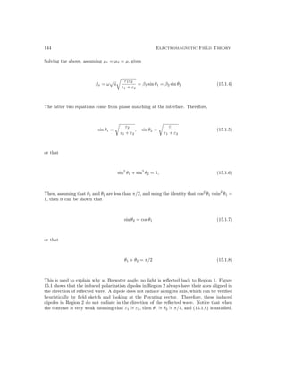
![Interesting Physical Phenomena 145
Figure 15.1: A figure showing a plane wave being reflected and transmitted at the Brewster’s
angle. In Region t, the polarization current or dipoles are all pointing in the kr direction, and
hence, there is no radiation in that direction (courtesy of J.A. Kong, EM Wave Theory [31]).
Because of the Brewster angle effect for TM polarization when ε2 = ε1, |RT M
| has to
go through a null when θi = θb. Therefore, |RT M
| ≤ |RT E
| as shown in Figure 15.2. Then
when a randomly polarized light is incident on a surface, the polarization where the electric
field is parallel to the surface (TE polarization) is reflected more than the polarization where
the magnetic field is parallel to the surface (TM polarization). This phenomenon is used to
design sun glasses to reduce road glare for drivers. For light reflected off a road surface, they
are predominantly horizontally polarized with respect to the surface of the road. When sun
glasses are made with vertical polarizers, they will filter out and mitigate the reflected rays
from the road surface to reduce road glare. This phenomenon can also be used to improve
the quality of photography by using a polarizer filter as shown in Figure 15.3.](https://image.slidesharecdn.com/emftall20191204-240115133321-d13ecad1/85/EMFTAll2-159-320.jpg)
![146 Electromagnetic Field Theory
Figure 15.2: Because |RT M
| has to through a null when θi = θb, therefore, |RT M
| ≤ |RT E
|
for all θi as shown above.
Figure 15.3: Because the TM and TE lights will be reflected differently, polarizer filter can
produce remarkable effects on the quality of the photograph [96].
15.1.2 Surface Plasmon Polariton
Surface plasmon polariton occurs for the same mathematical reason for the Brewster angle
effect but the physical mechanism is quite different. Many papers and textbooks will introduce
this phenomenon from a different angle. But here, we will introduce it from the Fresnel
reflection coefficient for the TM waves.
The reflection coefficient RT M
can become infinite if ε2 0, which is possible in a plasma
medium. In this case, the criterion for the denominator to be zero is
−ε2β1z = ε1β2z (15.1.9)
When the above is satisfied, RT M
becomes infinite. This implies that a reflected wave exists
when there is no incident wave. Or Href = HincRT M
, and when RT M
= ∞, Hinc can be](https://image.slidesharecdn.com/emftall20191204-240115133321-d13ecad1/85/EMFTAll2-160-320.jpg)
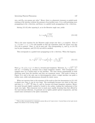
![148 Electromagnetic Field Theory
Figure 15.4: Figure showing a surface plasmonic mode propagating at an air-plasma interface.
As in all resonant systems, a resonant mode entails the exchange of energies. In the case
of surface plasmonic resonance, the energy is exchanged between the kinetic energy of the
electrons and the energy store in the electic field (courtesy of Wikipedia [99]).
15.2 Homomorphism of Uniform Plane Waves and Trans-
mission Lines Equations
It turns out that the plane waves through layered medium can be mapped into the multi-
section transmission line problem due to mathematical homomorphism between the two prob-
lems. Hence, we can kill two birds with one stone: apply all the transmission line techniques
and equations that we have learnt to solve for the solutions of waves through layered medium
problems.2
For uniform plane waves, since they are proportional to exp(−jβ · r), we know that with
∇ → −jβ, Maxwell’s equations becomes
β × E = ωµH (15.2.1)
β × H = −ωεE (15.2.2)
for a general isotropic homogeneous medium. We will specialize these equations for different
polarizations.
15.2.1 TE or TEz Waves
For this, one assumes a TE wave traveling in z direction with electric field polarized in the y
direction, or E = ŷEy, H = x̂Hx + ẑHz, then we have from (15.2.1)
βzEy = −ωµHx (15.2.3)
βxEy = ωµHz (15.2.4)
2This treatment is not found elsewhere, and is peculiar to these lecture notes.](https://image.slidesharecdn.com/emftall20191204-240115133321-d13ecad1/85/EMFTAll2-162-320.jpg)
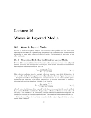
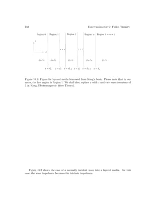
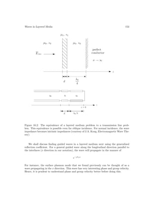
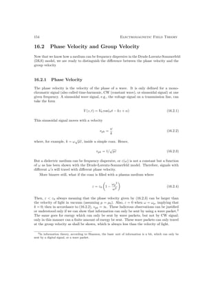
![Waves in Layered Media 155
16.2.2 Group Velocity
Figure 16.3: A Gaussian wave packet can be thought of as a linear superposition of monochro-
matic waves of slightly different frequencies. If one Fourier transforms the above signal, it
will be a narrow-band signal centered about certain ω0 (courtesy of Wikimedia [100]).
Now, consider a narrow band wave packet as shown in Figure 16.3. It cannot be mono-
chromatic, but can be written as a linear superposition of many frequencies. One way to
express this is to write this wave packet as an integral in terms of Fourier transform, or a
summation over many frequencies, namely
V (z, t) =
∞
−∞
dωV (z, ω)ejωt
(16.2.5)
Assume that V (z, t) is the solution to the dispersive transmission line equations with ε(ω),
then it can be shown that V (z, ω) is the solution to the one-dimensional Helmholtz equation3
d2
dz2
V (z, ω) + k2
(ω)V (z, ω) = 0 (16.2.6)
3In this notes, we will use k and β interchangeably for wavenumber. The transmission line community
tends to use β while the optics community uses k.](https://image.slidesharecdn.com/emftall20191204-240115133321-d13ecad1/85/EMFTAll2-169-320.jpg)
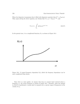
![Waves in Layered Media 157
Figure 16.5: The frequency spectrum of V0(ω).
Thus, we can approximate the integrand in the vicinity of ω = ω0, and let
k(ω) ∼
= k(ω0) + (ω − ω0)
dk(ω0)
dω
+
1
2
(ω − ω0)2 d2
k(ω0)
dω2
+ · · · (16.2.8)
To ensure the real-valuedness of (16.2.5), one ensures that −ω part of the integrand is exactly
the complex conjugate of the +ω part. Another way is to sum over only the +ω part of the
integral and take twice the real part of the integral. So, for simplicity, we write (16.2.5) as
V (z, t) = 2e
∞
0
dωV0(ω)ej(ωt−kz)
(16.2.9)
Since we need to integrate over ω ≈ ω0, we can substitute (16.2.8) into (16.2.9) and rewrite
it as
V (z, t) ∼
= 2e
ej[ω0t−k(ω0)z]
∞
0
dωV0(ω)ej(ω−ω0)t
e−j(ω−ω0) dk
dω z
| {z }
F (t− dk
dω z)
(16.2.10)
where more specifically,
F
t −
dk
dω
z
=
∞
0
dωV0(ω)ej(ω−ω0)t
e−j(ω−ω0) dk
dω z
(16.2.11)](https://image.slidesharecdn.com/emftall20191204-240115133321-d13ecad1/85/EMFTAll2-171-320.jpg)
![158 Electromagnetic Field Theory
It can be seen that the above integral now involves the integral summation over a small range
of ω in the vicinity of ω0. By a change of variable by letting Ω = ω − ω0, it becomes
F
t −
dk
dω
z
=
+∆
−∆
dΩV0(Ω + ω0)ejΩ(t− dk
dω z) (16.2.12)
When Ω ranges from −∆ to +∆ in the above integral, the value of ω ranges from ω0 − ∆ to
ω0 + ∆. It is assumed that outside this range of ω, V0(ω) is sufficiently small so that its value
can be ignored.
The above itself is a Fourier transform integral that involves only the low frequencies of
the Fourier spectrum. Hence, F is a slowly varying function. Moreover, this function F moves
with a velocity
vg =
dω
dk
(16.2.13)
Here, F(t− z
vg
) in fact is the velocity of the envelope in Figure 16.3. In (16.2.10), the envelope
function F(t − z
vg
) is multiplied by the rapidly varying function
ej[ω0t−k(ω0)z]
(16.2.14)
before one takes the real part of the entire function. Hence, this rapidly varying part represents
the rapidly varying carrier frequency shown in Figure 16.3. More importantly, this carrier,
the rapidly varying part of the signal, moves with the velocity
vph =
ω0
k(ω0)
(16.2.15)
which is the phase velocity.
16.3 Wave Guidance in a Layered Media
Now that we have understood phase and group velocity, we are at ease with studying the
We have seen that in the case of a surface plasmonic resonance, the wave is guided by an
interface because the Fresnel reflection coefficient becomes infinite. This physically means that
a reflected wave exists even if an incident wave is absent or vanishingly small. This condition
can be used to find a guided mode in a layered medium, namely, to find the condition under
which the generalized reflection coefficient (16.1.2) will become infinite.
16.3.1 Transverse Resonance Condition
Therefore, to have a guided mode exist in a layered medium, the denominator of (16.1.2) is
zero, or that
1 + R12R̃23e−2jβ2zl2
= 0 (16.3.1)](https://image.slidesharecdn.com/emftall20191204-240115133321-d13ecad1/85/EMFTAll2-172-320.jpg)

![Lecture 17
Dielectric Waveguides
Before we embark on the study of dielectric waveguides, we will revisit the transverse reso-
nance again. The transverse resonance condition allows one to derive the guidance conditions
for a dielectric waveguide easily without having to match the boundary conditions at the
interface again: The boundary conditions are already used when deriving the Fresnel reflec-
tion coefficients, and hence they are embedded in these reflection coefficients. Much of the
materials in this lecture can be found in [31,38,75].
17.1 Generalized Transverse Resonance Condition
The guidance conditions, the transverse resonance condition given previously, can also be
derived for the more general case. The generalized transverse resonance condition is a powerful
condition that can be used to derive the guidance condition of a mode in a layered medium.
To derive this condition, we first have to realize that a guided mode in a waveguide is due
to the coherent or constructive interference of the waves. This implies that if a plane wave
starts at position 1 (see Figure 17.1)1
and is multiply reflected as shown, it will regain its
original phase in the x direction at position 5. Since this mode progresses in the z direction,
all these waves (also known as partial waves) are in phase in the z direction by the phase
matching condition. Otherwise, the boundary conditions cannot be satisfied. That is, waves
at 1 and 5 will gain the same phase in the z direction. But, for them to add coherently or
interfere coherently in the x direction, the transverse phase at 5 must be the same as 1.
Assuming that the wave starts with amplitude 1 at position 1, it will gain a transverse
phase of e−jβ0xt
when it reaches position 2. Upon reflection at x = x2, at position 3, the wave
becomes R̃+e−jβ0xt
where R̃+ is the generalized reflection coefficient at the right interface
of Region 0. Finally, at position 5, it becomes R̃−R̃+e−2jβ0xt
where R̃− is the generalized
reflection coefficient at the left interface of Region 0. For constructive interference to occur
1The waveguide convention is to assume the direction of propagation to be z. Since we are analyzing a
guided mode in a layered medium, z axis is as shown in this figure.
161](https://image.slidesharecdn.com/emftall20191204-240115133321-d13ecad1/85/EMFTAll2-175-320.jpg)
![162 Electromagnetic Field Theory
Figure 17.1: The transverse resonance condition for a layered medium. The phase of the wave
at position 5 should be equal to the transverse phase at position 1.
or for the mode to exist, we require that
R̃−R̃+e−2jβ0xt
= 1 (17.1.1)
The above is the generalized transverse resonance condition for the guidance condition for a
plane wave mode traveling in a layered medium.
In (17.1.1), a metallic wall has a reflection coefficient of 1 for a TM wave, hence if R̃+ is
1, Equation (17.1.1) becomes
1 − R̃−e2−jβ0xt
= 0. (17.1.2)
On the other hand, in (17.1.1), a metallic wall has a reflection coefficient of −1, for TE wave,
and Equation (17.1.1) becomes
1 + R̃−e2−jβ0xt
= 0. (17.1.3)
17.2 Dielectric Waveguide
The most important dielectric waveguide of the modern world is the optical fiber, whose
invention was credited to Charles Kao [90]. He was awarded the Nobel prize in 2009 [101].
However, the analysis of the optical fiber requires analysis in cylindrical coordinates and the
use of special functions such as Bessel functions. In order to capture the essence of dielectric
waveguides, one can study the slab dielectric waveguide, which shares many salient features
with the optical fiber. This waveguide is also used as thin-film optical waveguides (see Figure
17.2). We start with analyzing the TE modes in this waveguide.](https://image.slidesharecdn.com/emftall20191204-240115133321-d13ecad1/85/EMFTAll2-176-320.jpg)
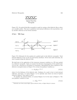
![164 Electromagnetic Field Theory
Also, we assume that ε1 ε0 so that total internal reflection occurs at both interfaces as
the wave bounces around so that β0x = −jα0x. Therefore, for TE polarization, the single-
interface reflection coefficient is
R10 =
µ0β1x − µ1β0x
µ0β1x + µ1β0x
=
µ0β1x + jµ1α0x
µ0β1x − jµ1α0x
= ejθT E
(17.2.3)
where θT E is the Goos-Hanschen shift for total internal reflection. It is given by
θT E = 2 tan−1
µ1α0x
µ0β1x
(17.2.4)
The guidance condition for constructive interference according to (17.2.1) is such that
2θT E − 2β1xd = 2nπ (17.2.5)
From the above, dividing it by four, and taking its tangent, we get
tan
θT E
2
= tan
nπ
2
+
β1xd
2
(17.2.6)
or
µ1α0x
µ0β1x
= tan
nπ
2
+
β1xd
2
(17.2.7)
The above gives rise to
µ1α0x = µ0β1x tan
β1xd
2
, n even (17.2.8)
−µ1α0x = µ0β1x cot
β1xd
2
, n odd (17.2.9)
It can be shown that when n is even, the mode profile is even, whereas when n is odd, the
mode profile is odd. The above can also be rewritten as
µ0
µ1
β1xd
2
tan
β1xd
2
=
α0xd
2
, even modes (17.2.10)
−
µ0
µ1
β1xd
2
cot
β1xd
2
=
α0xd
2
, odd modes (17.2.11)
Using the fact that −α2
0x = β2
0 − β2
z , and that β2
1x = β2
1 − β2
z , eliminating βz from these two
equations, one can show that
α0x = [ω2
(µ11 − µ00) − β2
1x]
1
2 (17.2.12)](https://image.slidesharecdn.com/emftall20191204-240115133321-d13ecad1/85/EMFTAll2-178-320.jpg)
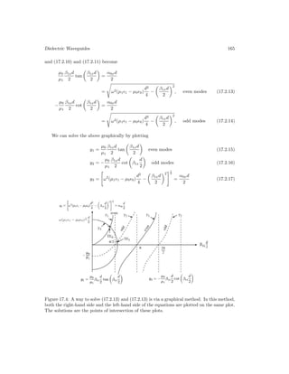
![166 Electromagnetic Field Theory
In the above, y3 is the equation of a circle; the radius of the circle is given by
ω(µ1–1 − µ0–0)
1
2
d
2
. (17.2.18)
The solutions to (17.2.13) and (17.2.14) are given by the intersections of y3 with y1 and
y2. We note from (17.2.1) that the radius of the circle can be increased in three ways: (i)
by increasing the frequency, (ii) by increasing the contrast µ1„1
µ0„0
, and (iii) by increasing the
thickness d of the slab.3
The mode profiles of the first two modes are shown in Figure 17.5.
Figure 17.5: Mode profiles of the TE0 and TE1 modes of a dielectric slab waveguide (courtesy
of J.A. Kong [31]).
When β0x = −jα0x, the reflection coefficient for total internal reflection is
RT E
10 =
µ0β1x + jµ1α0x
µ0β1x − jµ1α0x
= exp
+2j tan−1
µ1α0x
µ0β1x
(17.2.19)
and
RT E
10
= 1. Hence, the wave is guided by total internal reflections.
Cut-off occurs when the total internal reflection ceases to occur, i.e. when the frequency
decreases such that α0x = 0.
From Figure 17.4, we see that α0x = 0 when
ω(µ1–1 − µ0–0)
1
2
d
2
=
mπ
2
, m = 0, 1, 2, 3, . . . (17.2.20)
3These features are also shared by the optical fiber.](https://image.slidesharecdn.com/emftall20191204-240115133321-d13ecad1/85/EMFTAll2-180-320.jpg)
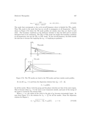
![168 Electromagnetic Field Theory
Hence the group and phase velocities approach that of the dielectric slab. This is because
when ω → ∞, α0x → ∞, implying that the fields are trapped or confined in the slab and
propagating within it. Because of this, the dispersion diagram of the different modes appear
as shown in Figure 17.7. In this figure,4
kc1, kc2, and kc3 are the cut-off wave number or
frequency of the first three modes. Close to cut-off, the field is traveling mostly outside
the waveguide, and kz ≈ ω
√
µ0ε0, and both the phase and group velocities approach that
of the outer medium as shown in the figure. When the frequency increases, the mode is
tightly confined in the dielectric slab, and kz ≈ ω
√
µ1ε1. Both the phase and group velocities
approach that of Region 1 as shown.
Figure 17.7: Here, we have kz versus k1 plot for dielectric slab waveguide. Near its cut-off,
the energy of the mode is in the outer region, and hence, its group velocity is close to that of
the outer region. At high frequencies, the mode is tightly bound to the slab, and its group
velocity approaches that of the dielectric slab (courtesy of J.A. Kong [31]).
17.2.2 TM Case
For the TM case, a similar guidance condition analogous to (17.2.1) can be derived but with
the understanding that the reflection coefficients in (17.2.1) are now TM reflection coefficients.
4Please note again that in this course, we will use β and k interchangeably for wavenumbers.](https://image.slidesharecdn.com/emftall20191204-240115133321-d13ecad1/85/EMFTAll2-182-320.jpg)
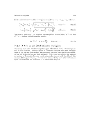

![Lecture 18
Hollow Waveguides
Hollow waveguides are useful for high-power microwaves. Air has a higher breakdown voltage
compared to most materials, and hence, could be a good medium for propagating high power
microwave. Also, hollow waveguides are sufficiently shielded from the rest of the world so
that interference from other sources is minimized. Furthermore, for radio astronomy, they
can provide a low-noise system immune to interference. Air generally has less loss than
materials, and loss is often the source of thermal noise. A low loss waveguide is also a low
noise waveguide.1
Many waveguide problems can be solved in closed form. An example is the coaxial waveg-
uide previously discussed. But there are many other waveguide problems that have closed
form solutions. Closed form solutions to Laplace and Helmholtz equations are obtained by the
separation of variables method. The separation of variables method works only for separable
coordinate systems. (There are 11 separable coordinates for Helmholtz equations, but 13 for
Laplace equation.) Some examples of separable coordinate systems are cartesian, cylindrical,
and spherical coordinates. But these three coordinates are about all we need to know for
solving many engineering problems. More complicated cases are now handled with numerical
methods using computers.
When a waveguide has a center conductor or two conductors like a coaxial cable, it can
support a TEM wave where both the electric field and the magnetic field are orthogonal to
the direction of propagation. The uniform plane wave is an example of a TEM wave, for
instance.
However, when the waveguide is hollow or is filled completely with a homogeneous medium,
without a center conductor, it cannot support a TEM mode as we shall prove next. Much of
the materials of this lecture can be found in [31,75,84].
1There is a fluctuation dissipation theorem [102, 103] that says that when a system loses energy to the
environment, it also receives the same amount of energy from the environment in order to conserve energy.
Hence, a lossy system loses energy to its environment, but it receives energy back from the environment in
terms of thermal noise.
171](https://image.slidesharecdn.com/emftall20191204-240115133321-d13ecad1/85/EMFTAll2-185-320.jpg)
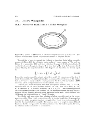
![Hollow Waveguides 173
18.1.2 TE Case (Ez = 0, Hz 6= 0)
In this case, the field inside the waveguide is TE to z or TEz. To ensure a TE field, we can
write the E field as
E(r) = ∇ × ẑΨh(r) (18.1.2)
Equation (18.1.2) will guarantee that Ez = 0 due to its construction. Here, Ψh(r) is a scalar
potential and ẑ is called the pilot vector.2
The waveguide is assumed source free and filled with a lossless, homogeneous material.
Eq. (18.1.2) also satisfies the source-free condition since ∇·E = 0. And hence, from Maxwell’s
equations, it can be shown that the electric field E(r) satisfies the following Helmholtz wave
equation, or partial differential equation that
(∇2
+ β2
)E(r) = 0 (18.1.3)
where β2
= ω2
µε. Substituting (18.1.2) into (18.1.3), we get
(∇2
+ β2
)∇ × ẑΨh(r) = 0 (18.1.4)
In the above, we assume that ∇2
∇ × ẑΨ = ∇ × ẑ(∇2
Ψ), or that these operators commute.3
Then it follows that
∇ × ẑ(∇2
+ β2
)Ψh(r) = 0 (18.1.5)
Thus, if Ψh(r) satisfies the following Helmholtz wave equation of partial differential equa-
tion
(∇2
+ β2
)Ψh(r) = 0 (18.1.6)
then (18.1.5) is satisfied, and so is (18.1.3). Hence, the E field constructed with (18.1.2)
satisfies Maxwell’s equations, if Ψh(r) satisfies (18.1.6).
2It “pilots” the field so that it is transverse to z.
3This is a mathematical parlance, and a commutator is defined to be [A, B] = AB − BA for two operators
A and B. If these two operators commute, then [A, B] = 0.](https://image.slidesharecdn.com/emftall20191204-240115133321-d13ecad1/85/EMFTAll2-187-320.jpg)
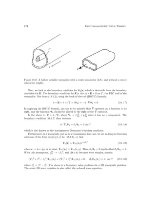
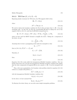
![176 Electromagnetic Field Theory
18.2 Rectangular Waveguides
Rectangular waveguides are among the simplest waveguides to analyze because closed form
solutions exist in cartesian coordinates. One can imagine traveling waves in the xy directions
bouncing off the walls of the waveguide causing standing waves to exist inside the waveguide.
As shall be shown, it turns out that not all electromagnetic waves can be guided by
a hollow waveguide. Only when the wavelength is short enough, or the frequency is high
enough that an electromagnetic wave can be guided by a waveguide. When a waveguide
mode cannot propagate in a waveguide, that mode is known to be cut-off. The concept of
cut-off for hollow waveguide is quite different from that of a dielectric waveguide we have
learned previously.
18.2.1 TE Modes (H Mode or Hz = 0 Mode)
For this mode, the scalar potential Ψhs(rs) satisfies
(∇s
2
+ βs
2
)Ψhs(rs) = 0,
∂
∂n
Ψhs(rs) = 0 on C (18.2.1)
where βs
2
= β2
− βz
2
. A viable solution using separation of variables4
for Ψhs(x, y) is then
Ψhs(x, y) = A cos(βxx) cos(βyy) (18.2.2)
where βx
2
+ β2
y = β2
s . One can see that the above is the representation of standing waves
in the xy directions. It is quite clear that Ψhs(x, y) satisfies equation (18.2.1). Furthermore,
cosine functions, rather than sine functions are chosen with the hindsight that the above
satisfies the homogenous Neumann boundary condition at x = 0, and y = 0 surfaces.
Figure 18.3: The schematic of a rectangular waveguide. By convention, the length of the
longer side is usually named a.
4For those who are not familiar with this topic, please consult p. 385 of Kong [31].](https://image.slidesharecdn.com/emftall20191204-240115133321-d13ecad1/85/EMFTAll2-190-320.jpg)
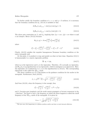
![178 Electromagnetic Field Theory
When ω ωmn,c, the TEmn mode is evanescent and cannot propagate inside the waveguide.
A corresponding cutoff wavelength is then
λmn,c =
2
[ m
a
2
+ n
b
2
]1/2
(18.2.11)
So when λ λmn,c, the mode cannot propagate inside the waveguide.
When m = n = 0, then Ψh(r) = Ψhs(x, y) exp(∓jβzz) is a function independent of x and
y. Then E(r) = ∇ × ẑΨh(r) = ∇s × ẑΨh(r) = 0. It turns out the only way for Hz 6= 0 is for
H(r) = ẑH0 which is a static field in the waveguide. This is not a very interesting mode, and
thus TE00 propagating mode is assumed not to exist and not useful. So the TEmn modes
cannot have both m = n = 0. As such, the TE10 mode, when a b, is the mode with the
lowest cutoff frequency or longest cutoff wavelength.
For the TE10 mode, for the mode to propagate, from (18.2.11), it is needed that
λ λ10,c = 2a (18.2.12)
The above has the nice physical meaning that the wavelength has to be smaller than 2a in
order for the mode to fit into the waveguide. As a mnemonic, we can think that photons have
“sizes”, corresponding to its wavelength. Only when its wavelength is small enough can the
photons go into (or be guided by) the waveguide. The TE10 mode, when a b, is also the
mode with the lowest cutoff frequency or longest cutoff wavelength.
It is seen with the above analysis, when the wavelength is short enough, or frequency is
high enough, many modes can be guided. Each of these modes has a different group and
phase velocity. But for most applications, a single guided mode only is desirable. Hence,
the knowledge of the cutoff frequencies of the fundamental mode (the mode with the lowest
cutoff frequency) and the next higher mode is important. This allows one to pick a frequency
window within which only a single mode can propagate in the waveguide.
It is to be noted that when a mode is cutoff, the field is evanescent, and there is no real
power flow down the waveguide: Only reactive power is conveyed by such a mode.](https://image.slidesharecdn.com/emftall20191204-240115133321-d13ecad1/85/EMFTAll2-192-320.jpg)
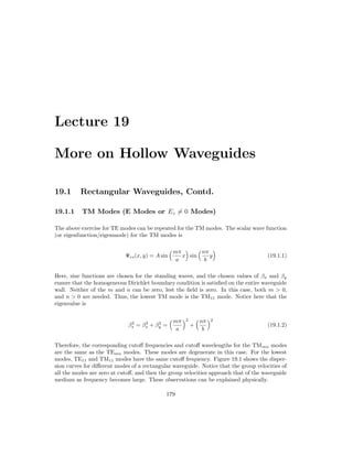
![180 Electromagnetic Field Theory
Figure 19.1: Dispersion curves for a rectangular waveguide. Notice that the lowest TM mode
is the TM11 mode, and k is equivalent to β in this course (courtesy of J.A. Kong [31]).
19.1.2 Bouncing Wave Picture
We have seen that the transverse variation of a mode in a rectangular waveguide can be
expanded in terms of sine and cosine functions which represent standing waves, or that they
are
[exp(−jβxx) ± exp(jβxx)] [exp(−jβyy) ± exp(jβyy)]
When the above is expanded and together with the exp(−jβzz) the mode propagating in the
z direction, we see four waves bouncing around in the xy directions and propagating in the z
direction. The picture of this bouncing wave can be depicted in Figure 19.2.
Figure 19.2: The waves in a rectangular waveguide can be thought of as bouncing waves off
the four walls as they propagate in the z direction.](https://image.slidesharecdn.com/emftall20191204-240115133321-d13ecad1/85/EMFTAll2-194-320.jpg)
![More on Hollow Waveguides 181
19.1.3 Field Plots
Plots of the fields of different rectangular waveguide modes are shown in Figure 19.3. Higher
frequencies are needed to propagate the higher order modes or the high m and n modes.
Notice that for higher m’s and n’s, the transverse wavelengths are getting shorter, implying
that βx and βy are getting larger because of the higher frequencies involved.
Notice also how the electric field and magnetic field curl around each other. Since ∇×H =
jωεE and ∇ × E = −jωµH, they do not curl around each other “immediately” but with a
π/2 phase delay due to the jω factor. Therefore, the E and H fields do not curl around each
other at one location, but at a displaced location due to the π/2 phase difference. This is
shown in Figure 19.4.
Figure 19.3: Transverse field plots of different modes in a rectangular waveguide (courtesy
of Andy Greenwood. Original plots published in Lee, Lee, and Chuang, IEEE T-MTT, 33.3
(1985): pp. 271-274. [104]).](https://image.slidesharecdn.com/emftall20191204-240115133321-d13ecad1/85/EMFTAll2-195-320.jpg)
![182 Electromagnetic Field Theory
Figure 19.4: Field plot of a mode propagating in the z direction of a rectangular waveguide.
Notice that the E and H fields do not exactly curl around each other.
19.2 Circular Waveguides
Another waveguide where closed-form solutions can be easily obtained is the circular hollow
waveguide as shown in Figure 19.5.
Figure 19.5: Schematic of a circular waveguide.
19.2.1 TE Case
For a circular waveguide, it is best first to express the Laplacian operator, ∇s
2
= ∇s · ∇s, in
cylindrical coordinates. Such formulas are given in [31, 105]. Doing a table lookup, ∇sΨ =](https://image.slidesharecdn.com/emftall20191204-240115133321-d13ecad1/85/EMFTAll2-196-320.jpg)
![More on Hollow Waveguides 183
ρ̂ ∂
∂ρ Ψ + φ̂1
ρ
∂
∂φ , ∇s · A = 1
ρ
∂
∂ρ ρAρ + 1
ρ
∂
∂φ Aφ. Then
∇s
2
+ βs
2
Ψhs =
1
ρ
∂
∂ρ
ρ
∂
∂ρ
+
1
ρ2
∂2
∂φ2
+ βs
2
Ψhs(ρ, φ) = 0 (19.2.1)
The above is the partial differential equation for field in a circular waveguide. Using separation
of variables, we let
Ψhs(ρ, φ) = Bn(βsρ)e±jnφ
(19.2.2)
Then ∂2
∂φ2 → −n2
, and (19.2.1) becomes an ordinary differential equation which is
1
ρ
d
dρ
ρ
d
dρ
−
n2
ρ2
+ βs
2
Bn(βsρ) = 0 (19.2.3)
Here, we can let βsρ in (19.2.2) and (19.2.3) be x. Then the above can be rewritten as
1
x
d
dx
x
d
dx
−
n2
x2
+ 1
Bn(x) = 0 (19.2.4)
The above is known as the Bessel equation whose solutions are special functions denoted as
Bn(x).
These special functions are Jn(x), Nn(x), H
(1)
n (x), and H
(2)
n (x) which are called Bessel,
Neumann, Hankel function of the first kind, and Hankel function of the second kind, respec-
tively, where n is the order, and x is the argument.1
Since this is a second order ordinary
differential equation, it has only two independent solutions. Therefore, two of the four com-
monly encountered solutions of Bessel equation are independent. Therefore, they can be
expressed then in term of each other. Their relationships are shown below:2
Bessel, Jn(x) =
1
2
[Hn
(1)
(x) + Hn
(2)
(x)] (19.2.5)
Neumann, Nn(x) =
1
2j
[Hn
(1)
(x) − Hn
(2)
(x)] (19.2.6)
Hankel–First kind, Hn
(1)
(x) = Jn(x) + jNn(x) (19.2.7)
Hankel–Second kind, Hn
(2)
(x) = Jn(x) − jNn(x) (19.2.8)
It can be shown that
Hn
(1)
(x) ∼
r
2
πx
ejx−j(n+ 1
2 ) π
2 , x → ∞ (19.2.9)
Hn
(2)
(x) ∼
r
2
πx
e−jx+j(n+ 1
2 ) π
2 , x → ∞ (19.2.10)
They correspond to traveling wave solutions when x = βsρ → ∞. Since Jn(x) and Nn(x)
are linear superpositions of these traveling wave solutions, they correspond to standing wave
1Some textbooks use Yn(x) for Neumann functions.
2Their relations with each other are similar to those between exp(−jx), sin(x), and cos(x).](https://image.slidesharecdn.com/emftall20191204-240115133321-d13ecad1/85/EMFTAll2-197-320.jpg)
![184 Electromagnetic Field Theory
solutions. Moreover, Nn(x), Hn
(1)
(x), and Hn
(2)
(x) → ∞ when x → 0. Since the field has to
be regular when ρ → 0 at the center of the waveguide shown in Figure 19.5, the only viable
solution for the waveguide is that Bn(βsρ) = AJn(βsρ). Thus for a circular hollow waveguide,
the eigenfunction or mode is of the form
Ψhs(ρ, φ) = AJn(βsρ)e±jnφ
(19.2.11)
To ensure that the eigenfunction and the eigenvalue are unique, boundary condition for the
partial differential equation is needed. The homogeneous Neumann boundary condition on
the PEC waveguide wall then translates to
d
dρ
Jn(βsρ) = 0, ρ = a (19.2.12)
Defining Jn
0
(x) = d
dx Jn(x), the above is the same as
Jn
0
(βsa) = 0 (19.2.13)
Plots of Bessel functions and their derivatives are shown in Figure 19.6. The above are the
zeros of the derivative of Bessel function and they are tabulated in many textbooks. The
m-th zero of Jn
0
(x) is denoted to be βnm in many books,3
and some of them are also shown
in Figure 19.7; and hence, the guidance condition for a waveguide mode is then
βs = βnm/a (19.2.14)
for the TEnm mode. From the above, β2
s can be obtained which is the eigenvalue of (19.2.1)
and (19.2.3). Using the fact that βz =
p
β2 − β2
s , then βz will become pure imaginary if β2
is small enough so that β2
β2
s or β βs. From this, the corresponding cutoff frequency of
the TEnm mode is
ωnm,c =
1
√
µε
βnm
a
(19.2.15)
When ω ωnm,c, the corresponding mode cannot propagate in the waveguide as βz becomes
pure imaginary. The corresponding cutoff wavelength is
λnm,c =
2π
βnm
a (19.2.16)
By the same token, when λ λnm,c, the corresponding mode cannot be guided by the
waveguide. It is not exactly precise to say this, but this gives us the heuristic notion that if
wavelength or “size” of the wave or photon is too big, it cannot fit inside the waveguide.
3Notably, Abramowitz and Stegun, Handbook of Mathematical Functions [106]. An online version is
available at [107].](https://image.slidesharecdn.com/emftall20191204-240115133321-d13ecad1/85/EMFTAll2-198-320.jpg)
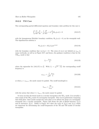
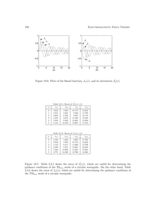
![More on Hollow Waveguides 187
Figure 19.8: Transverse field plots of different modes in a circular waveguide (courtesy of
Andy Greenwood. Original plots published in Lee, Lee, and Chuang [104]).](https://image.slidesharecdn.com/emftall20191204-240115133321-d13ecad1/85/EMFTAll2-201-320.jpg)

![Lecture 20
More on Waveguides and
Transmission Lines
20.1 Circular Waveguides, Contd.
As in the rectangular waveguide case, the guidance of the wave in a circular waveguide can
be viewed as bouncing waves in the radial direction. But these bouncing waves give rise
to standing waves expressible in terms of Bessel functions. The scalar potential (or pilot
potential) for the modes in the waveguide is expressible as
Ψαs(ρ, φ) = AJn(βsρ)e±jnφ
(20.1.1)
where α = h for TE waves and α = e for TM waves. The Bessel function or wave is expressible
in terms of Hankel functions as in (19.2.5). Since Hankel functions are traveling waves, Bessel
functions represent standing waves. Therefore, the Bessel waves can be thought of as bouncing
traveling waves as in the rectangular waveguide case. In the azimuthal direction, one can
express e±jnφ
as traveling waves in the φ direction, or they can be expressed as cos(nφ) and
sin(nφ) which are standing waves in the φ direction.
20.1.1 An Application of Circular Waveguide
When a real-world waveguide is made, the wall of the metal waveguide is not made of perfect
electric conductor, but with some metal of finite conductivity. Hence, tangential E field is
not zero on the wall, and energy can dissipate into the waveguide wall. It turns out that due
to symmetry, the TE01 mode of a circular waveguide has the lowest loss of all the waveguide
modes including rectangular waveguide modes. Hence, this waveguide mode is of interest to
astronomers who are interested in building low-loss and low-noise systems.1
The TE01 mode has electric field given by E = φ̂Eφ. Furthermore, looking at the magnetic
field, the current is mainly circumferential flowing in the φ direction. Moreover, by looking
1Low-loss systems are also low-noise due to energy conservation and the fluctuation dissipation theorem
[102,103,108].
189](https://image.slidesharecdn.com/emftall20191204-240115133321-d13ecad1/85/EMFTAll2-203-320.jpg)
![190 Electromagnetic Field Theory
at a bouncing wave picture of the guided waveguide mode, this mode has a small component
of tangential magnetic field on a waveguide wall: It becomes increasingly smaller as the
frequency increases (see Figure 20.1).
Figure 20.1: Bouncing wave picture of the Bessel wave inside a circular waveguide for the
TE01 mode.
The tangential magnetic field needs to be supported by a surface current on the waveguide
wall. This implies that the surface current on the waveguide wall becomes smaller as the
frequency increases. The wall loss (or copper loss or eddy current loss) of the waveguide,
hence, becomes smaller for higher frequencies. In fact, for high frequencies, the TE01 mode
has the smallest copper loss of the waveguide modes: It becomes the mode of choice (see
Figure 20.2). Waveguides supporting the TE01 modes are used to connect the antennas of
the very large array (VLA) for detecting extra-terrestrial signals in radio astronomy [109] as
shown in Figure 20.3.](https://image.slidesharecdn.com/emftall20191204-240115133321-d13ecad1/85/EMFTAll2-204-320.jpg)
![More on Waveguides and Transmission Lines 191
Figure 20.2: Losses of different modes in a circular waveguide . It is seen that at high
frequencies, the TE01 mode has the lowest loss (courtesy of [110]).](https://image.slidesharecdn.com/emftall20191204-240115133321-d13ecad1/85/EMFTAll2-205-320.jpg)
![192 Electromagnetic Field Theory
Figure 20.3: Picture of the Very Large Array (courtesy of [109]).
Figure 20.4 shows two ways of engineering a circular waveguide so that the TE01 mode
is enhanced: (i) by using a mode filter that discourages the guidance of other modes but
not the TE01 mode, and (ii), by designing ridged waveguide wall to discourage the flow of
axial current and hence, the propagation of the non-TE01 mode. More details of circular
waveguides can be found in [110]. Typical loss of a circular waveguide can be as low as 2
dB/km.
As shall be learnt later, an open circular waveguide can be made into an aperture antenna
quite easily, because the fields of the aperture are axially symmetric. Such antenna is called a
horn antenna. Because of this, the radiation pattern of such an antenna is axially symmetric,
which can be used to produce axially symmetric circularly polarized (CP) waves. Ways to
enhance the TE01 mode are also desirable [111] as shown in Figure 20.5.](https://image.slidesharecdn.com/emftall20191204-240115133321-d13ecad1/85/EMFTAll2-206-320.jpg)
![More on Waveguides and Transmission Lines 193
Figure 20.4: Ways to enhance the TE01 mode in a circular waveguide. Such waveguide is
used in astronomy such as designing the communication between antennas in a very large
array (VLA [109]), or it is used in a circular horn antenna [111].](https://image.slidesharecdn.com/emftall20191204-240115133321-d13ecad1/85/EMFTAll2-207-320.jpg)
![194 Electromagnetic Field Theory
Figure 20.5: Picture of a circular horn antenna where corrugated wall is used to enhance the
TE01 mode (courtesy of [112]).
20.2 Remarks on Quasi-TEM Modes, Hybrid Modes,
and Surface Plasmonic Modes
We have analyzed some simple structures where closed form solutions are available. These
solutions offer physical insight into how waves are guided, and how they are cutoff from
guidance. As has been shown, for some simple waveguides, the modes can be divided into
TEM, TE, and TM modes. However, most waveguides are not simple. We will remark on
various complexities that arise in real world applications.
20.2.1 Quasi-TEM Modes
Figure 20.6: Some examples of practical coaxial-like waveguides (left), and the optical fiber
(right). The environment of these waveguides is an inhomogeneous medium, and hence, a
pure TEM mode cannot propagate on these waveguides.](https://image.slidesharecdn.com/emftall20191204-240115133321-d13ecad1/85/EMFTAll2-208-320.jpg)
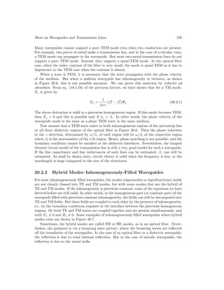
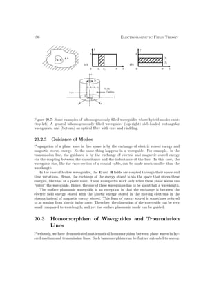
![More on Waveguides and Transmission Lines 197
uides and transmission lines. We can show this first for TE modes in a hallow waveguide,
and the case for TM modes can be established by invoking duality principle.2
20.3.1 TE Case
For this case, Ez = 0, and from Maxwell’s equations
∇ × H = jωεE (20.3.1)
By letting ∇ = ∇s + ∇z, H = Hs + Hz where ∇z = ẑ ∂
∂z , and Hz = ẑHz, and the subscript
s implies transverse to z components, then
(∇s + ∇z) × (Hs + Hz) = ∇s × Hs + ∇z × Hs + ∇s × Hz (20.3.2)
where it is understood that ∇z × Hz = 0. Notice that the first term on the right-hand side
of the above is pointing in the z direction. Therefore, by letting E = Es + Ez, and equating
transverse components in (20.3.1), we have3
∇z × Hs + ∇s × Hz = jωεEs (20.3.3)
To simplify the above equation, we shall remove Hz from above. Next, from Faraday’s law,
we have
∇ × E = −jωµH (20.3.4)
Again, by letting E = Es + Ez, we can show that (20.3.4) can be written as
∇s × Es + ∇z × Es + ∇s × Ez = −jωµ(Hs + Hz) (20.3.5)
Equating z components of the above, we have
∇s × Es = −jωµHz (20.3.6)
Using (20.3.6), Eq.(20.3.3) can be rewritten as
∇z × Hs + ∇s ×
1
−jωµ
∇s × Es = +jωεEs (20.3.7)
The above can be further simplified by noting that
∇s × ∇s × Es = ∇s(∇s · Es) − ∇s · ∇sEs (20.3.8)
But since ∇ · E = 0, and Ez = 0 for TE modes, it implies that ∇s · Es = 0. Also, from
Maxwell’s equations, we have previously shown that for a homogeneous source-free medium,
(∇2
+ β2
)E = 0 (20.3.9)
2I have not seen exposition of such mathematical homomorphism elsewhere except in very simple cases [31].
3And from the above, it is obvious that ∇s × Hs = jωεEz, but this equation will not be used in the
subsequent derivation.](https://image.slidesharecdn.com/emftall20191204-240115133321-d13ecad1/85/EMFTAll2-211-320.jpg)
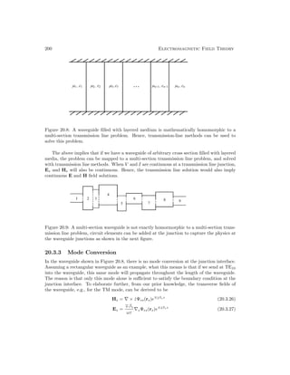
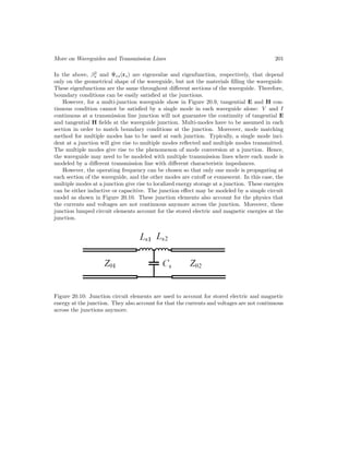

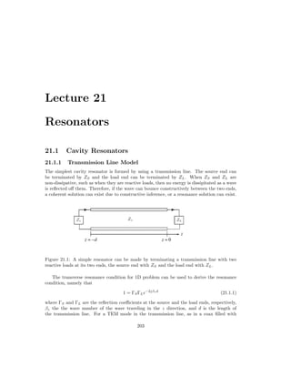
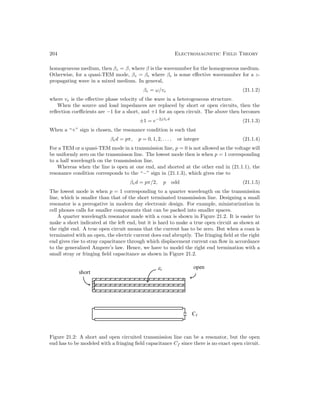
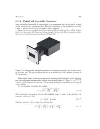
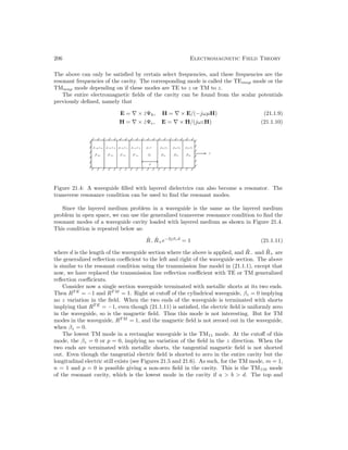
![Resonators 207
side views of the fields of this mode is shown in Figures 21.5 and 21.6. The corresponding
resonant frequency of this mode satisfies the equation
ω2
110
c2
=
π
a
2
+
π
b
2
(21.1.12)
Figure 21.5: The top view of the E and H fields of a rectangular resonant cavity.
Figure 21.6: The side view of the E and H fields of a rectangular resonant cavity (courtesy
of J.A. Kong [31]).
For the TE modes, it is required that p = 0, otherwise, the field is zero in the cavity. For
example, it is possible to have the TE101 mode.
ω2
101
c2
=
π
a
2
+
π
d
2
(21.1.13)
Clearly, this mode has a higher resonant frequency compared to the TM110 mode if d b.](https://image.slidesharecdn.com/emftall20191204-240115133321-d13ecad1/85/EMFTAll2-221-320.jpg)
![208 Electromagnetic Field Theory
The above analysis can be applied to circular and other cylindrical waveguides with βs
determined differently. For instance, for a circular waveguide, βs is determined differently
using Bessel functions, and for a general arbitrarily shaped waveguide, βs may be determined
numerically.
Figure 21.7: A circular resonant cavity made by terminating a circular waveguide (courtesy
of Kong [31]).
For a spherical cavity, one would have to analyze the problem in spherical coordinates.
The equations will have to be solved by separation of variables using spherical harmonics.
Details are given on p. 468 of Kong [31].
21.2 Some Applications of Resonators
Resonators in microwaves and optics can be used for designing filters, energy trapping devices,
and antennas. As filters, they are used like LC resonators in circuit theory. A concatenation
of them can be used to narrow or broaden the bandwidth of a filter. As an energy trapping
device, a resonator can build up a strong field inside the cavity if it is excited with energy
close to its resonance frequency. They can be used in klystrons and magnetrons as microwave
sources, a laser cavity for optical sources, or as a wavemeter to measure the frequency of
the electromagnetic field at microwave frequencies. An antenna is a radiator that we will
discuss more fully later. The use of a resonator can help in resonance tunneling to enhance
the radiation efficiency of an antenna.](https://image.slidesharecdn.com/emftall20191204-240115133321-d13ecad1/85/EMFTAll2-222-320.jpg)
![Resonators 209
21.2.1 Filters
Microstrip line resonators are often used to make filters. Transmission lines are often used to
model microstrip lines in a microwave integrated circuits (MIC). In MIC, due to the etching
process, it is a lot easier to make an open circuit rather than a short circuit. But a true open
circuit is hard to make as an open ended microstrip line has fringing field at its end as shown
in Figure 21.8 [113, 114]. The fringing field gives rise to fringing field capacitance as shown
in Figure 21.2. Then the appropriate ΓS and ΓL can be used to model the effect of fringing
field capacitance. Figure 21.9 shows a concatenation of two microstrip resonators to make
a microstrip filter. This is like using a concatenation of LC tank circuits to design filters in
circuit theory.
Figure 21.8: End effects and junction effects in a microwave integrated circuit [113, 114]
(courtesy of Microwave Journal).
Figure 21.9: A microstrip filter designed using concatenated resonators. The connectors to
the coax cable are the SMA (sub-miniature type A) connectors (courtesy of aginas.fe.up.pt).](https://image.slidesharecdn.com/emftall20191204-240115133321-d13ecad1/85/EMFTAll2-223-320.jpg)
![210 Electromagnetic Field Theory
Optical filters can be made with optical etalon as in a Fabry-Perot resonator, or concate-
nation of them. This is shown in Figure 21.10.
Figure 21.10: Design of a Fabry-Perot resonator [50,75,115,116].
21.2.2 Electromagnetic Sources
Microwave sources are often made by transferring kinetic energy from an electron beam
to microwave energy. Klystrons, magnetrons, and traveling wave tubes are such devices.
However, the cavity resonator in a klystron enhances the interaction of the electrons with the
microwave field, causing the field to grow in amplitude as shown in Figure 21.11.](https://image.slidesharecdn.com/emftall20191204-240115133321-d13ecad1/85/EMFTAll2-224-320.jpg)
![Resonators 211
Figure 21.11: A klystron works by converting the kinetic energy of an electron beam into the
energy of a traveling microwave next to the beam (courtesy of Wiki [117]).
Magnetron cavity works also by transferring the kinetic energy of the electron into the
microwave energy. By injecting hot electrons into the magnetron cavity, the cavity resonance
is magnified by the kinetic energy from the hot electrons, giving rise to microwave energy.
Figure 21.12: A magnetron works by having a high-Q microwave cavity resonator. When the
cavity is injected with energetic electrons from the cathode to the anode, the kinetic energy
of the electron feeds into the energy of the microwave (courtesy of Wiki [118]).
Figure 21.13 shows laser cavity resonator to enhance of light wave interaction with material](https://image.slidesharecdn.com/emftall20191204-240115133321-d13ecad1/85/EMFTAll2-225-320.jpg)
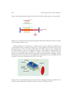
![Resonators 213
21.2.3 Frequency Sensor
Because a cavity resonator can be used as an energy trap, it will siphon off energy from
a microwave waveguide when it hits the resonance frequency of the passing wave in the
waveguide. This can be used to determine the frequency of the passing wave. Wavemeters
are shown in Figure 21.15 and 21.16.
Figure 21.15: An absorption wave meter can be used to measure the frequency of microwave
(courtesy of Wiki [119]).](https://image.slidesharecdn.com/emftall20191204-240115133321-d13ecad1/85/EMFTAll2-227-320.jpg)
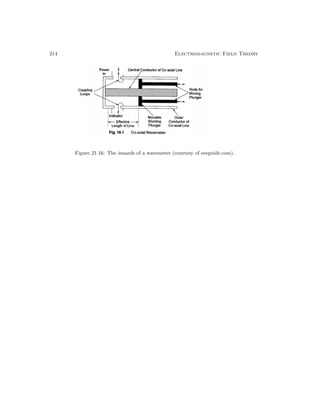
![Lecture 22
Quality Factor of Cavities, Mode
Orthogonality
22.1 The Quality Factor of a Cavity
22.1.1 General Concepts
The quality factor of a cavity or its Q measures how ideal or lossless a cavity resonator is.
An ideal lossless cavity resonator will sustain free oscillations forever, while most resonators
sustain free oscillations for a finite time due to losses coming from radiation, or dissipation in
the dielectric material filling the cavity, or resistive loss of the metallic part of the cavity. Be-
cause of losses, the free oscillation in a cavity has electromagnetic field with time dependence
as follows:
E ∝ e−αt
cos(ωt + φ1), H ∝ e−αt
cos(ωt + φ2) (22.1.1)
The total time-average stored energy, which is proportional to 1
4 |E|
2
+ 1
4 µ |H|
2
is of the form
hWT i = hWEi + hWHi = W0e−2αt
(22.1.2)
If there is no loss, hWT i will remain constant. However, with loss, the average stored energy
will decrease to e−1
of its original value at t = 1
2α . The Q of a cavity is a measure of the
number of free oscillations the field would have before the energy stored decreases to e−1
of
its original value (see Figure 22.1). In a time interval t = 1
2α , the number of free oscillations
in radians is ωt or ω
2α ; hence, the Q is defined to be [31]
Q =
ω
2α
(22.1.3)
215](https://image.slidesharecdn.com/emftall20191204-240115133321-d13ecad1/85/EMFTAll2-229-320.jpg)
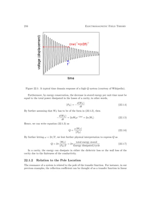
![Quality Factor of Cavities, Mode Orthogonality 217
system theory: The input is the incident wave, while the output is the reflected wave. If
we encounter the resonance of the system at a particular frequency, the reflection coefficient
becomes infinite. This infinite value can be modeled by a pole of the transfer function in the
complex ω plane. In other words, in the vicinity of the pole in the frequency domain,
R(ω) ∼
A
ω − ωp
(22.1.8)
In principle, when ω = ωp, the reflection coefficient becomes infinite, but this does not
happen in practice due to loss in the system. In other words, ωp is not a real number and the
pole does not lie on the real ω axis; the pole is displaced slightly off the real axis to account
for loss. In fact, it is quite easy to show that the pole is at ωp = ω0 +jα.1
Then the full-width
half maximum (FWHM) bandwidth is ∆ω = 2α, and the Q can be written as
Q = ω0/∆ω (22.1.9)
Typical plots of transfer function versus frequency for a system with different Q’s are shown
in Figure 22.2.
Figure 22.2: A typical system response versus frequency for different Q’s (courtesy of al-
laboutcircuits.com).
1It is quite easy to show that the Fourier inverse transform of the above corresponds to a decaying sinusoid
[45].](https://image.slidesharecdn.com/emftall20191204-240115133321-d13ecad1/85/EMFTAll2-231-320.jpg)
![218 Electromagnetic Field Theory
22.1.3 Some Formulas for Q for a Metallic Cavity
If the cavity is filled with air, then, the loss comes mainly from the metallic loss or copper-loss
from the cavity wall. In this case, the power dissipated on the wall is given by [31]
hPDi =
1
2
e
S
(E × H∗
) · n̂ dS =
1
2
e
S
(n̂ × E) · H∗
dS (22.1.10)
where S is the surface of the cavity wall.2
Here, (n̂ × E) is the tangential component of the
electric field which would have been zero if the cavity wall is made of ideal PEC. Also, n̂
is taken to be the outward pointing normal at the surface S. However, for metallic walls,
n̂ × E = HtZm where Zm is the intrinsic impedance for the metallic conductor, viz., Zm =
q
µ
εm
≈
q
µ
−j σ
ω
=
pωµ
2σ (1 + j),3
where we have assumed that εm ≈ −jσ
ω , and Ht is the
tangential magnetic field. This relation between E and H will ensure that power is flowing
into the metallic surface. Hence,
hPDi =
1
2
e
S
r
ωµ
2σ
(1 + j) |Ht|
2
dS =
1
2
r
ωµ
2σ S
|Ht|
2
dS (22.1.11)
By further assuming that the stored electric and magnetic energies of a cavity are equal
to each other at resonance, the stored energy can be obtained by
hWT i =
1
2
µ
V
|H|2
dV (22.1.12)
Written explicitly, the Q becomes
Q =
p
2ωµσ
V
|H|
2
dV
S
|Ht|
2
dS
=
2
δ
V
|H|
2
dV
S
|Ht|
2
dS
(22.1.13)
In the above, δ is the skin depth of the metallic wall. Hence, the more energy stored we can
have with respect to the power dissipated, the higher the Q of a resonating system. The lower
the metal loss, or the smaller the skin depth, the higher the Q would be.
Notice that in (22.1.13), the numerator is a volume integral and hence, is proportional to
volume, while the denominator is a surface integral and is proportional to surface. Thus, the
Q, a dimensionless quantity, is roughly proportional to
Q ∼
V
Sδ
(22.1.14)
where V is the volume of the cavity, while S is its surface area. From the above, it is noted
that a large cavity compared to its skin depth has a larger Q than an small cavity.
2We have used the cyclic identity that a · (b × c) = b · (c × a) = c · (a × b) in the above (see Some Useful
Mathematical Formulas).
3When an electromagnetic wave enters a conductive region with a large β, it can be shown that the wave
is refracted to propagate normally to the surface, and hence, this formula can be applied.](https://image.slidesharecdn.com/emftall20191204-240115133321-d13ecad1/85/EMFTAll2-232-320.jpg)
![220 Electromagnetic Field Theory
22.2 Mode Orthogonality and Matrix Eigenvalue Prob-
lem
It turns out that the modes of a waveguide or a resonator are orthogonal to each other. This
is intimately related to the orthogonality of eigenvectors of a matrix operator.4
Thus, it is
best to understand this by the homomorphism between the electromagnetic mode problem
and the matrix eigenvalue problem. Because of this similarity, electromagnetic modes are also
called eigenmodes. Thus it is prudent that we revisit the matrix eigenvalue problem (EVP).
22.2.1 Matrix Eigenvalue Problem (EVP)
It is known in matrix theory that if a matrix is hermitian, then its eigenvalues are all real.
Furthermore, their eigenvectors with distinct eigenvalues are orthogonal to each other [69].
Assume that an eigenvalue and an eigenvector exists for the hermitian matrix A. Then
A · vi = λivi (22.2.1)
Dot multiplying the above from the left by v†
i where † indicates conjugate transpose, then
the above becomes
v†
i · A · vi = λiv†
i · vi (22.2.2)
Since A is hermitian, then the quantity v†
i ·A·vi is purely real. Moreover, the quantity v†
i ·vi
is positive real. So in order for the above to be satisfied, λi has to be real.
To prove orthogonality of eigenvectors, now, assume that A has two eigenvectors with
distinct eigenvalues such that
A · vi = λivi (22.2.3)
A · vj = λjvj (22.2.4)
Left dot multiply the first equation with v†
j and do the same to the second equation with v†
i ,
one gets
v†
j · A · vi = λiv†
j · vi (22.2.5)
v†
i · A · vj = λjv†
i · vj (22.2.6)
Taking the conjugate transpose of (22.2.5) in the above, and since A is hermitian, their left-
hand sides (22.2.5) and (22.2.6) become the same. Subtracting the two equations, we arrive
at
0 = (λi − λj)v†
j · vi (22.2.7)
For distinct eigenvalues, λi 6= λj, the only way for the above to be satisfied is that
v†
j · vi = Ciδij (22.2.8)
Hence, eigenvectors of a hermitian matrix with distinct eigenvalues are orthogonal to each
other. The eigenvalues are also real.
4This mathematical homomorphism is not discussed in any other electromagnetic textbooks.](https://image.slidesharecdn.com/emftall20191204-240115133321-d13ecad1/85/EMFTAll2-234-320.jpg)
![Quality Factor of Cavities, Mode Orthogonality 221
22.2.2 Homomorphism with the Waveguide Mode Problem
We shall next show that the problem for finding the waveguide modes or eigenmodes is
analogous to the matrix eigenvalue problem. The governing equation for a waveguide mode
is BVP involving the reduced wave equation previously derived, or
∇2
sψi(rs) + β2
isψi(rs) = 0 (22.2.9)
with the pertinent homogeneous Dirichlet or Neumann boundary condition,F depending on
if TE or TM modes are considered. In the above, the differential operator ∇2
s is analogous to
the matrix operator A, the eigenfunction ψi(rs) is analogous to the eigenvector vi, and β2
is
is analogous to the eigenvalue λi.
Discussion on Functional Space
To think of a function ψ(rs) as a vector, one has to think in the discrete world.5
If one needs
to display the function ψ(rs), on a computer, one will evaluate the function ψ(rs) at discrete
N locations rls, where l = 1, 2, 3, . . . , N. For every rls or every l, there is a scalar number
ψ(rls). These scalar numbers can be stored in a column vector in a computer indexed by l.
The larger N is, the better is the discrete approximation of ψ(rs). In theory, one needs N to
be infinite to describe this function exactly.6
From the above discussion, a function is analogous to a vector and a functional space
is analogous to a vector space. However, a functional space is infinite dimensional. But in
order to compute on a computer with finite resource, such functions are approximated with
vectors. Infinite dimensional vector spaces are replaced with finite dimensional ones to make
the problem computable. Such infinite dimensional functional space is also called Hilbert
space.
It is also necessary to define the inner product between two vectors in a functional space
just as inner product between two vectors in an matrix vector space. The inner product (or
dot product) between two vectors in matrix vector space is
vt
i · vj =
N
X
l=1
vi,lvj,l (22.2.10)
The analogous inner product between two vectors in function space is7
hψi, ψji =
S
drsψi(rs)ψj(rs) (22.2.11)
where S denotes the cross-sectional area of the waveguide over which the integration is per-
formed. The left-hand side is the shorthand notation for inner product in functional space or
the infinite dimensional Hilbert space.
5Some of these concepts are discussed in [34,120].
6In mathematical parlance, the index for ψ(rs) is uncountably infinite or nondenumerable.
7In many math books, the conjugation of the first function ψi is implied, but here, we follow the electro-
magnetic convention that the conjugation of ψi is not implied unless explicitly stated.](https://image.slidesharecdn.com/emftall20191204-240115133321-d13ecad1/85/EMFTAll2-235-320.jpg)
![222 Electromagnetic Field Theory
Another requirement for a vector in a functional Hilbert space is that it contains finite
energy or that
Ef =
S
drs|ψi(rs)|2
(22.2.12)
is finite. The above is analogous to that for a matrix vector v as
Em =
N
X
l=1
|vl|2
(22.2.13)
The square root of the above is often used to denote the “length” or the “metric” of the
vector. Finite energy also implies that the vectors are of finite length. This length is also
called the “norm” of a vector.
22.2.3 Proof of Orthogonality of Waveguide Modes
Because of the aforementioned discussion, we see the similarity between a function Hilbert
space, and the matrix vector space. In order to use the result of the matrix EVP, one key
step is to prove that the operator ∇2
s is hermitian. In matrix algebra, a matrix operator is
hermitian if
x†
i · A · xj =
x†
j · A
†
· xi
†
=
x†
j · A · xi
†
=
x†
j · A · xi
∗
(22.2.14)
The first equality follows from standard matrix algebra,8
the second equality follows if A =
A
†
, or that A is hermitian. The last equality follows because the quantity in the parenthesis
is a scalar, and hence, its conjugate transpose is just its conjugate.
By the same token, a functional operator ∇2
s is hermitian if
hψ∗
i , ∇2
sψji =
S
drsψ∗
i (rs)∇2
sψj(rs) = (hψ∗
j , ∇2
sψii)∗
=
S
drsψj(rs)∇2
sψ∗
i (rs) (22.2.15)
Using integration by parts for higher dimensions and with the appropriate boundary condition
for the function ψ(rs), the above equality can be proved.
To this end, one uses the identity that
∇s · [ψ∗
i (rs)∇sψj(rs)] = ψ∗
i (rs)∇2
sψj(rs) + ∇sψ∗
i (rs) · ∇sψj(rs) (22.2.16)
Integrating the above over the cross sectional area S, and invoking Gauss divergence theorem
in 2D, one gets that
C
dln̂ · (ψ∗
i (rs)∇sψj(rs)) =
S
drs ψ∗
i (rs)∇2
sψj(rs)
+
S
drs (∇ψ∗
i (rs) · ∇sψj(rs)) (22.2.17)
8(A · B · C)† = C
†
· B
†
· A
†
[69].](https://image.slidesharecdn.com/emftall20191204-240115133321-d13ecad1/85/EMFTAll2-236-320.jpg)
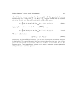

![228 Electromagnetic Field Theory
Equation (23.1.20) is known as the Lorenz gauge3
and the above equations are Helmholtz
equations with source terms. Not only are these equations simplified, they can be solved
independently of each other since they are decoupled from each other.
Equations (23.1.21) and (23.1.22) can be solved using the Green’s function method. Equa-
tion (23.1.21) actually implies three scalar equations for the three x, y, z components, namely
that
∇2
Ai + ω2
µεAi = −µJi (23.1.23)
where i above can be x, y, or z. Therefore, (23.1.21) and (23.1.22) together constitute
four scalar equations similar to each other. Hence, we need only to solve their point-source
response, or the Green’s function of these equations by solving
∇2
g(r, r0
) + β2
g(r, r0
) = −δ(r − r0
) (23.1.24)
where β2
= ω2
µε.
Previously, we have shown that when β = 0,
g(r, r0
) = g(|r − r0
|) =
1
4π|r − r0|
When β 6= 0, the correct solution is
g(r, r0
) = g(|r − r0
|) =
e−jβ|r−r0
|
4π|r − r0|
(23.1.25)
which can be verified by back substitution.
By using the principle of linear superposition, or convolution, the solutions to (23.1.21)
and (23.1.22) are then
A(r) = µ
dr0
J(r0
)
e−jβ|r−r0
|
4π|r − r0|
(23.1.26)
Φ(r) =
1
ε
dr0
%(r0
)
e−jβ|r−r0
|
4π|r − r0|
(23.1.27)
In the above dr0
is the shorthand notation for dx dy dz and hence, they are still volume
integrals.
23.1.4 More on Scalar and Vector Potentials
It is to be noted that Maxwell’s equations are symmetrical and this is especially so when we
add a magnetic current M to Maxwell’s equations and magnetic charge %m to Gauss’s law.4
Then the equations become
∇ × E = −jωµH − M (23.1.28)
∇ × H = jωεE + J (23.1.29)
∇ · µH = %m (23.1.30)
∇ · εE = % (23.1.31)
3Please note that this Lorenz is not the same as Lorentz.
4In fact, Maxwell exploited this symmetry [121].](https://image.slidesharecdn.com/emftall20191204-240115133321-d13ecad1/85/EMFTAll2-242-320.jpg)
![Scalar and Vector Potentials 229
The above can be solved in two stages, using the principle of linear superposition. First, we
can set M = 0 and %m = 0 and solve for the fields as we have done. Second, we can set J = 0
and % = 0 and solve for the fields next. Then the total general solution is just the linear
superposition of these two solutions.
For the second case, we can define an electric vector potential F such that
D = −∇ × F (23.1.32)
and a magnetic scalar potential Φm such that
H = −∇Φm − jωF (23.1.33)
By invoking duality principle, one can gather that [41]
F(r) = ε
dr0
M(r0
)
e−jβ|r−r0
|
4π|r − r0|
(23.1.34)
Φm(r) =
1
µ
dr0
%m(r0
)
e−jβ|r−r0
|
4π|r − r0|
(23.1.35)
As mentioned before, even though magnetic sources do not exist, they can be engineered.
In many engineering designs, it is more expeditious to think magnetic sources to enrich the
diversity of electromagnetic technologies.
23.2 When is Static Electromagnetic Theory Valid?
We have learnt in the previous section that for electrodynamics,
E = −∇Φ − jωA (23.2.1)
where the second term above on the right-hand side is due to induction, or the contribution
to the electric field from the time-varying magnetic filed. Hence, much things we learn in
potential theory that E = −∇Φ is not exactly valid. But simple potential theory that E =
−∇Φ is very useful because of its simplicity. We will study when static electromagnetic theory
can be used to model electromagnetic systems. Since the third and the fourth Maxwell’s
equations are derivable from the first two, let us first study when we can ignore the time
derivative terms in the first two of Maxwell’s equations, which, in the frequency domain, are
∇ × E = −jωµH (23.2.2)
∇ × H = jωεE + J (23.2.3)
When the terms multiplied by jω above can be ignored, then electrodynamics can be replaced
with static electromagnetics, which are much simpler. That is why Ampere’s law, Coulomb’s
law, and Gauss’ law were discovered first. Quasi-static electromagnetic theory eventually
gave rise to circuit theory and telegraphy technology. Circuit theory consists of elements like
resistors, capacitors, and inductors. Given that we have now seen electromagnetic theory in](https://image.slidesharecdn.com/emftall20191204-240115133321-d13ecad1/85/EMFTAll2-243-320.jpg)
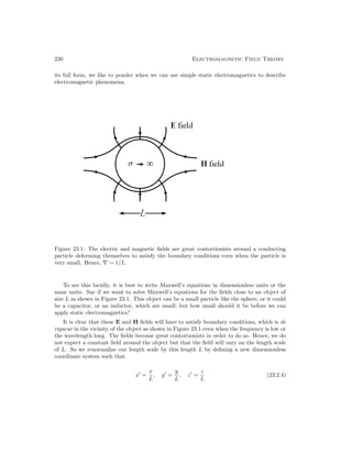
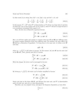
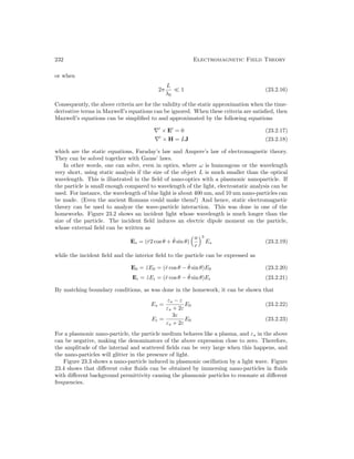
![Scalar and Vector Potentials 233
Figure 23.2: A plane electromagnetic wave incident on a particle. When the particle size is
small compared to wavelength, static analysis can be used to solve this problem (courtesy of
Kong [31]).
Figure 23.3: A nano-particle undergoing electromagnetic oscillation when an electromagnetic
wave impinges on it (courtesy of sigmaaldric.com).](https://image.slidesharecdn.com/emftall20191204-240115133321-d13ecad1/85/EMFTAll2-247-320.jpg)
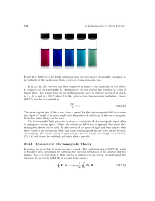
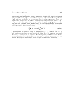

![Lecture 24
Circuit Theory Revisited
24.1 Circuit Theory Revisited
Circuit theory is one of the most successful and often used theories in electrical engineering.
Its success is mainly due to its simplicity: it can capture the physics of highly complex
circuits and structures, which is very important in the computer and micro-chip industry.
Now, having understood electromagnetic theory in its full glory, it is prudent to revisit circuit
theory and study its relationship to electromagnetic theory [29,31,48,59].
The two most important laws in circuit theory are Kirchoff current law (KCL) and Kirch-
hoff voltage law (KVL) [14, 45]. These two laws are derivable from the current continuity
equation and from Faraday’s law.
24.1.1 Kirchhoff Current Law
Figure 24.1: Schematics showing the derivation of Kirchhoff current law. All currents flowing
into a node must add up to zero.
237](https://image.slidesharecdn.com/emftall20191204-240115133321-d13ecad1/85/EMFTAll2-251-320.jpg)
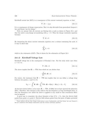
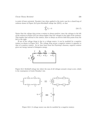
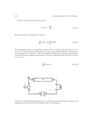
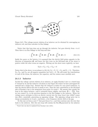
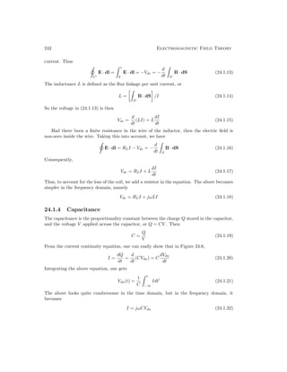
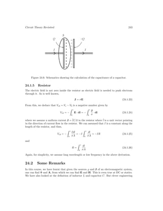
![244 Electromagnetic Field Theory
is driven by heuristics: it is better, at times, to look at inductors and capacitors as energy
storage devices, rather than flux linkage and charge storage devices.
Another important remark is that even though circuit theory is simpler that Maxwell’s
equations in its full glory, not all the physics is lost in it. The physics of the induction
term in Faraday’s law and the displacement current term in generalized Ampere’s law are
still retained. In fact, wave physics is still retained in circuit theory: one can make slow
wave structure out a series of inductors and capacitors. The lumped-element model of a
transmission line is an example of a slow-wave structure design. Since the wave is slow, it has
a smaller wavelength, and resonators can be made smaller: We see this in the LC tank circuit
which is a much smaller resonator in wavelength compared to a microwave cavity resonator
for instance. The only short coming is that inductors and capacitors generally have higher
losses than air or vacuum.
24.2.1 Energy Storage Method for Inductor and Capacitor
Often time, it is more expedient to think of inductors and capacitors as energy storage devices.
This enables us to identify stray (also called parasitic) inductances and capacitances more
easily. This manner of thinking allows for an alternative way of calculating inductances and
capacitances as well [29].
The energy stored in an inductor is due to its energy storage in the magnetic field, and it
is alternatively written, according to circuit theory, as
Wm =
1
2
LI2
(24.2.1)
Therefore, it is simpler to think that an inductance exists whenever there is stray magnetic
field to store magnetic energy. A piece of wire carries a current that produces a magnetic
field enabling energy storage in the magnetic field. Hence, a piece of wire in fact behaves
like a small inductor, and it is non-negligible at high frequencies: Stray inductances occur
whenever there are stray magnetic fields.
By the same token, a capacitor can be thought of as an electric energy storage device
rather than a charge storage device. The energy stored in a capacitor, from circuit theory, is
We =
1
2
CV 2
(24.2.2)
Therefore, whenever stray electric field exists, one can think of stray capacitances as we have
seen in the case of fringing field capacitances in a microstrip line.
24.2.2 Finding Closed-Form Formulas for Inductance and Capaci-
tance
Finding closed form solutions for inductors and capacitors is a difficult endeavor. Only certain
geometries are amenable to closed form solutions. Even a simple circular loop does not have
a closed form solution for its inductance L. If we assume a uniform current on a circular
loop, in theory, the magnetic field can be calculated using Bio-Savart law that we have learnt](https://image.slidesharecdn.com/emftall20191204-240115133321-d13ecad1/85/EMFTAll2-258-320.jpg)
![Circuit Theory Revisited 245
before, namely that
H(r) =
I(r
)dl
× R̂
4πR2
(24.2.3)
But the above cannot be evaluated in closed form save in terms of complicate elliptic integrals.
However, if we have a solenoid as shown in Figure 24.7, an approximate formula for the
inductance L can be found if the fringing field at the end of the solenoid can be ignored.
The inductance can be found using the flux linkage method [28, 29]. Figure 24.8 shows the
schematics used to find the approximate inductance of this inductor.
Figure 24.7: The flux-linkage method is used to estimate the inductor of a solenoid (courtesy
of SolenoidSupplier.Com).
Figure 24.8: Finding the inductor flux linkage by assuming the magnetic field is uniform
inside a long solenoid.
The capacitance of a parallel plate capacitor can be found by solving a boundary value
problem (BVP) for electrostatics. The electrostatic BVP for capacitor involves Poisson’s
equation and Laplace equation which are scalar equations [42][Thomson’s theorem].](https://image.slidesharecdn.com/emftall20191204-240115133321-d13ecad1/85/EMFTAll2-259-320.jpg)
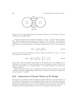
![Circuit Theory Revisited 247
Figure 24.10 shows the schematics and the cross section of a computer chip at different
levels: the transistor level at the bottom-most. The signals are taken out of a transistor by
XY lines at the middle level that are linked to the ball-grid array at the top-most level of
the chip. And then, the signal leaves the chip via a package. Since these nanometer-size
structures are much smaller than the wavelength, they are usually modeled by lumped R,
L, and C elements if retardation effect can be ignored. If retardation effect is needed, it is
usually modeled by a transmission line. This is important at the package level where the
dimensions of the components are larger.
A process of parameter extraction where computer software or field solvers (software that
solve Maxwell’s equations numerically) are used to extract these lumped-element parameters.
Finally, a computer chip is modeled as a network involving a large number of transistors,
diodes, and R, L, and C elements. Subsequently, a very useful commercial software called
SPICE (Simulation Program with Integrated-Circuit Emphasis) [122], which is a computer-
aided software, solves for the voltages and currents in this network.](https://image.slidesharecdn.com/emftall20191204-240115133321-d13ecad1/85/EMFTAll2-261-320.jpg)
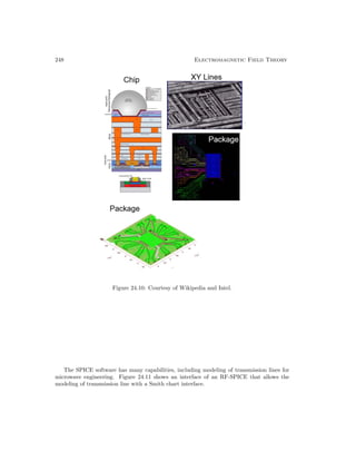
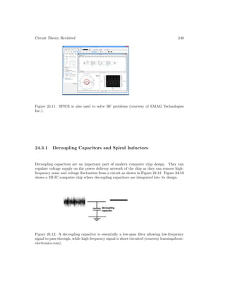
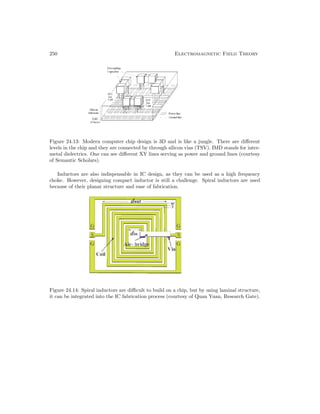
![Lecture 25
Radiation by a Hertzian Dipole
25.1 Radiation by a Hertzian Dipole
Radiation by arbitrary sources is an important problem for antennas and wireless communi-
cations. We will start with studying the Hertzian dipole which is the simplest of a radiation
source we can think of.
25.1.1 History
The original historic Hertzian dipole experiment is shown in Figure 25.1. It was done in 1887
by Heinrich Hertz [18]. The schematics for the original experiment is also shown in Figure
25.2.
A metallic sphere has a capacitance in closed form with respect to infinity or a ground
plane. Hertz could use those knowledge to estimate the capacitance of the sphere, and also,
he could estimate the inductance of the leads that are attached to the dipole, and hence, the
resonance frequency of his antenna. The large sphere is needed to have a large capacitance,
so that current can be driven through the wires. As we shall see, the radiation strength of
the dipole is proportional to p = ql the dipole moment. To get a large dipole moment, the
current flowing in the lead should be large.
251](https://image.slidesharecdn.com/emftall20191204-240115133321-d13ecad1/85/EMFTAll2-265-320.jpg)
![252 Electromagnetic Field Theory
Figure 25.1: Hertz’s original experiment on a small dipole (courtesy of Wikipedia [18]).
Figure 25.2: More on Hertz’s original experiment on a small dipole (courtesy of Wikipedia [18]
25.1.2 Approximation by a Point Source
A Hertzian dipole is a dipole which is much smaller than the wavelength under consideration
so that we can approximate it by a point current distribution, mathematically given by [31,38]
J(r) = ẑIlδ(r) (25.1.1)
The dipole may look like the following schematically. As long as we are not too close to the
dipole so that it does not look like a point source anymore, the above is a good model for a](https://image.slidesharecdn.com/emftall20191204-240115133321-d13ecad1/85/EMFTAll2-266-320.jpg)
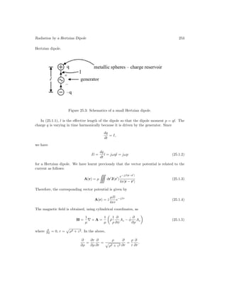
![254 Electromagnetic Field Theory
Hence,
H = −φ̂
ρ
r
Il
4π
−
1
r2
− jβ
1
r
e−jβr
(25.1.6)
Figure 25.4: Spherical coordinates are used to calculate the fields of a Hertzian dipole.
In spherical coordinates, ρ
r = sin θ, and (25.1.6) becomes [31]
H = φ̂
Il
4πr2
(1 + jβr)e−jβr
sin θ (25.1.7)
The electric field can be derived using Maxwell’s equations.
E =
1
jω–
∇ × H =
1
jω–
r̂
1
r sin θ
∂
∂θ
sin θHφ − θ̂
1
r
∂
∂r
rHφ
(25.1.8)
=
Ile−jβr
jω–4πr3
r̂2 cos θ(1 + jβr) + θ̂ sin θ(1 + jβr − β2
r2
) (25.1.9)
25.1.3 Case I. Near Field, βr 1
E ∼
=
p
4π–r3
(r̂2 cos θ + θ̂ sin θ), βr 1 (25.1.10)
H E, when βr 1 (25.1.11)
where p = ql is the dipole moment, and βr could be made very small by making r
λ small or
by making ω → 0. The above is like the static field of a dipole. The reason being that in](https://image.slidesharecdn.com/emftall20191204-240115133321-d13ecad1/85/EMFTAll2-268-320.jpg)
![Radiation by a Hertzian Dipole 255
the near field, the field varies rapidly, and space derivatives are much larger than the time
derivative.1
For instance,
∂
∂x
∂
c∂t
Alternatively, we can say that the above is equivalent to
∂
∂x
ω
c
or that
∇2
−
1
c2
∂2
∂t2
≈ ∇2
In other words, static theory prevails over dynamic theory.
25.1.4 Case II. Far Field (Radiation Field), βr 1
In this case,
E ∼
= θ̂jωµ
Il
4πr
e−jβr
sin θ (25.1.12)
and
H ∼
= φ̂jβ
Il
4πr
e−jβr
sin θ (25.1.13)
Note that Eθ
Hφ
= ωµ
β =
pµ
= η0. Here, E and H are orthogonal to each other and are both
orthogonal to the direction of propagation, as in the case of a plane wave. A spherical wave
resembles a plane wave in the far field approximation.
25.1.5 Radiation, Power, and Directive Gain Patterns
The time average power flow is given by
hSi =
1
2
e[E × H∗
] = r̂
1
2
η0 |Hφ|
2
= r̂
η0
2
βIl
4πr
2
sin2
θ (25.1.14)
The radiation field pattern of a Hertzian dipole is the plot of |E| as a function of θ at a
constant r. Hence, it is proportional to sin θ, and it can be proved that it is a circle.
1This is in agreement with our observation that electromagnetic fields are great contortionists: They will
deform themselves to match the boundary first before satisfying Maxwell’s equations. Since the source point
is very small, the fields will deform themselves so as to satisfy the boundary conditions near to the source
region. If this region is small compared to wavelength, the fields will vary rapidly over a small lengthscale
compared to wavelength.](https://image.slidesharecdn.com/emftall20191204-240115133321-d13ecad1/85/EMFTAll2-269-320.jpg)
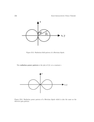
![Radiation by a Hertzian Dipole 257
The total power radiated by a Hertzian dipole is given by
P =
2π
0
dφ
π
0
dθr2
sin θhSri = 2π
π
0
dθ
η0
2
βIl
4π
2
sin3
θ (25.1.15)
Since
π
0
dθ sin3
θ = −
−1
1
(d cos θ)[1 − cos2
θ] =
1
−1
dx(1 − x2
) =
4
3
(25.1.16)
then
P =
4
3
πη0
βIl
4π
2
(25.1.17)
The directive gain of an antenna, G(θ, φ), is defined as [31]
G(θ, φ) =
hSri
P
4πr2
(25.1.18)
where
P
4πr2
is the power density if the power P were uniformly distributed over a sphere of radius r.
Substituting (25.1.14) and (25.1.17) into the above, we have
G(θ, φ) =
η0
2
βIl
4πr
2
sin2
θ
1
4πr2
4
3 η0π
βIl
4π
2 =
3
2
sin2
θ (25.1.19)
The peak of G(θ, φ) is known as the directivity of an antenna. It is 1.5 in the case of a
Hertzian dipole. If an antenna is radiating isotropically, its directivity is 1. Therefore, the
lowest possible values for the directivity of an antenna is 1, whereas it can be over 100 for
some antennas like reflector antennas (see Figure 25.7). A directive gain pattern is a plot
of the above function G(θ, φ) and it resembles the radiation power pattern.](https://image.slidesharecdn.com/emftall20191204-240115133321-d13ecad1/85/EMFTAll2-271-320.jpg)
![258 Electromagnetic Field Theory
Figure 25.7: The gain of a reflector antenna can be increased by deflecting the power radiated
in the desired direction by the use of a reflector (courtesy of racom.eu).
If the total power fed into the antenna instead of the total radiated power is used in the
denominator of (25.1.18), the ratio is known as the power gain or just gain. The total
power fed into the antenna is not equal to the total radiated power because there could be
some loss in the antenna system like metallic loss.
25.1.6 Radiation Resistance
Defining a radiation resistance Rr by P = 1
2 I2
Rr, we have [31]
Rr =
2P
I2
= η0
(βl)2
6π
≈ 20(βl)2
, where η0 = 377 ≈ 120π Ω (25.1.20)
For example, for a Hertzian dipole with l = 0.1λ, Rr ≈ 8Ω.
The above assumes that the current is uniformly distributed over the length of the Hertzian
dipole. This is true if there are two charge reservoirs at its two ends. For a small dipole with
no charge reservoir at the two ends, the currents have to vanish at the tip of the dipole as
shown in Figure 25.8.](https://image.slidesharecdn.com/emftall20191204-240115133321-d13ecad1/85/EMFTAll2-272-320.jpg)
![Radiation by a Hertzian Dipole 259
Figure 25.8: The current pattern on a short dipole can be approximated by a triangle since
the current has to be zero at the end points of the short dipole.
The effective length of the dipole is half of its actual length due to the manner the currents
are distributed. For example, for a half-wave dipole, a = λ
2 , and if we use leff = λ
4 in (25.1.20),
we have
Rr ≈ 50Ω (25.1.21)
However, a half-wave dipole is not much smaller than a wavelength and does not qualify to
be a Hertzian dipole. Furthermore, the current distribution on the half-wave dipole is not
triangular in shape as above. A more precise calculation shows that Rr = 73Ω for a half-wave
dipole [48].
The true current distribution on a half-wave dipole resembles that shown in Figure 25.9.
The current is zero at the end points, but the current has a more sinusoidal-like distribution
like that in a transmission line. In fact, one can think of a half-wave dipole as a flared,
open transmission line. In the beginning, this flared open transmission line came in the
form of biconical antennas which are shown in Figure 25.10 [123]. If we recall that the
characteristic impedance of a transmission line is
L/C, then as the spacing of the two
metal pieces becomes bigger, the equivalent characteristic impedance gets bigger. Therefore,
the impedance can gradually transform from a small impedance like 50 Ω to that of free
space, which is 377 Ω. This impedance matching helps mitigate reflection from the ends of
the flared transmission line, and enhances radiation.
Because of the matching nature of bicone antennas, they tend to have a broader band-
width, and are important in UWB (ultra-wide band) antennas [124].](https://image.slidesharecdn.com/emftall20191204-240115133321-d13ecad1/85/EMFTAll2-273-320.jpg)
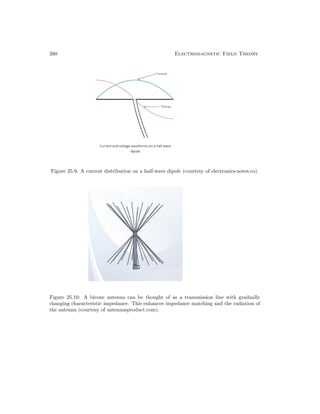
![Lecture 26
Radiation Fields, Far Fields
26.1 Radiation Fields or Far-Field Approximation
Figure 26.1:
In the previous lecture, we have derived the relation of the vector and scalar potentials to the
sources J and .1
They are given by
A(r) = µ
V
dr
J(r
)
e−jβ|r−r
|
4π|r − r|
(26.1.1)
Φ(r) =
1
ε V
dr
(r
)
e−jβ|r−r
|
4π|r − r|
(26.1.2)
1This topic is found in many standard textbooks in electromagnetics [31, 41, 48]. They are also found in
lecture notes [38,125].
261](https://image.slidesharecdn.com/emftall20191204-240115133321-d13ecad1/85/EMFTAll2-275-320.jpg)
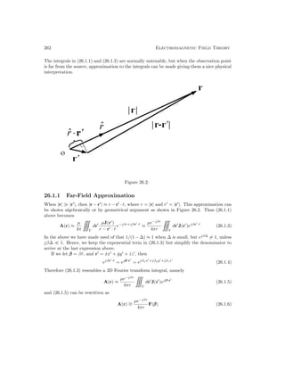
![Radiation Fields, Far Fields 263
where
F(β
β
β) =
V
dr0
J(r0
)ejβ·r0
(26.1.7)
is the 3D Fourier transform of J(r0
) with β = r̂β.
It is to be noted that this is not a normal 3D Fourier transform because |β|2
= βx
2
+βy
2
+
βz
2
= β2
. In other words, the length of the vector β is fixed to be β. In a normal 3D Fourier
transform, βx, βy, and βz are independent variables, with values in the range [−∞, ∞], and
βx
2
+ βy
2
+ βz
2
ranges from zero to infinity.
The above is the 3D “Fourier transform” of the current source J(r0
) with Fourier variables,
βx, βy, βz lying on a sphere of radius β and β
β
β = βr̂. This spherical surface in the Fourier
space is also called the Ewald’s sphere.
26.1.2 Locally Plane Wave Approximation
We can write r̂ or β
β
β in terms of direction cosines in spherical coordinates or that
r̂ = x̂ cos φ sin θ + ŷ sin φ sin θ + ẑ cos θ (26.1.8)
Hence,
F(β
β
β) = F(βr̂) = F(β, θ, φ) (26.1.9)
It is not truly a 3D function, since β is fixed. It is a 3D Fourier transform with data restricted
on a spherical surface.
Also in (26.1.6), when r r0
· r̂, e−jβr
is now a rapidly varying function of r while, F(β
β
β)
is only a slowly varying function of θ and φ, the observation angles. In other words, the
prefactor in (26.1.6), exp(−jβr)/r, can be thought of as resembling a spherical wave. Hence,
if one follows a ray of this spherical wave and moves in the r direction, the predominant
variation of the field is due to e−jβr
, whereas the direction of the vector β changes little, and
hence F(β) changes little. Furthermore, r0
in (26.1.7) are restricted to small or finite number,
making F(β) a weak function of β.
The above shows that in the far field, the wave radiated by a finite source resembles a
spherical wave. Moreover, a spherical wave resembles a plane wave when one is sufficiently
far from the source. Hence, we can write e−jβr
= e−jβ
β
β·r
where β
β
β = r̂β and r = r̂r so that a
spherical wave resembles a plane wave locally. This phenomenon is shown in Figure 26.3.](https://image.slidesharecdn.com/emftall20191204-240115133321-d13ecad1/85/EMFTAll2-277-320.jpg)
![264 Electromagnetic Field Theory
Figure 26.3: A spherical wave emanating from a source becomes locally a plane wave in the
far field.
Then, it is clear that with the plane-wave approximation, ∇ → −jβ
β
β = −jβr̂, and
H =
1
µ
∇ × A ≈ −j
β
µ
r̂ × (θ̂Aθ + φ̂Aφ) = j
β
µ
(θ̂Aφ − φ̂Aθ) (26.1.10)
Similarly [38,125],
E =
1
jωε
∇ × H ∼
= −j
β
ω
r̂ × H ∼
= −jω(θ̂Aθ + φ̂Aφ) (26.1.11)
Notice that β = βr̂ is orthogonal to E and H in the far field, a property of a plane wave.
Moreover, there are more than one way to derive the electric field E. Using (26.1.10) for the
magnetic field, the electric field can also be written as
E =
1
jωµε
∇ × ∇ × A (26.1.12)
Using the formula for the double-curl operator, the above can be rewritten as
E =
1
jωµε
∇∇ · A − ∇2
A
=
1
jωµε
−ββ + β2
I
· A (26.1.13)
where we have used that ∇2
A = −β2
A. Alternatively, we can factor β2
= ω2
µ and rewrite
the above as
E = −jω
−β̂β̂ + I
· A = −jω −r̂r̂ + I
· A (26.1.14)](https://image.slidesharecdn.com/emftall20191204-240115133321-d13ecad1/85/EMFTAll2-278-320.jpg)
![Radiation Fields, Far Fields 265
Since I = r̂r̂ + θ̂θ̂ + φ̂φ̂, then the above becomes
E = −jω
θ̂θ̂ + φ̂φ̂
· A = −jω(θ̂Aθ + φ̂Aφ) (26.1.15)
which is the same as previously derived. It also shows that the electric field is transverse to
the β vector. We can also arrive at the above by lettering E = −jωA − ∇Φ, and using the
appropriate formula for the scalar potential.
Furthermore, it can be shown that in the far field, using the plane-wave approximation,
|E|/|H| ≈ η (26.1.16)
where η is the intrinsic impedance of free space, which is a property of a plane wave. Moreover,
one can show that the time average Poynting’s vector in the far field is
hSi ≈
1
2η
|E|2
r̂ (26.1.17)
which resembles also the property of a plane wave. Since the radiated field is a spherical
wave, the Poynting’s vector is radial. Therefore,
hSi = r̂Sr(θ, φ) (26.1.18)
The plot of |E(θ, φ)| is termed the far-field pattern or the radiation pattern of an antenna or
the source, while the plot of |E(θ, φ)|2
is its far-field power pattern.
26.1.3 Directive Gain Pattern Revisited
Once the far-field power pattern Sr is known, the total power radiated by the antenna can
be found by
PT =
π
0
2π
0
r2
sin θdθdφSr(θ, φ) (26.1.19)
The above evaluates to a constant independent of r due to energy conservation. Now assume
that this same antenna is radiating isotropically in all directions, then the average power
density of this fictitious isotropic radiator as r → ∞ is
Sav =
PT
4πr2
(26.1.20)
A dimensionless directive gain pattern can be defined such that [31,125]
G(θ, φ) =
Sr(θ, φ)
Sav
=
4πr2
Sr(θ, φ)
PT
(26.1.21)
The above function is independent of r in the far field since Sr ∼ 1/r2
in the far field. As in
the Hertzian dipole case, the directivity of an antenna D = max(G(θ, φ)), is the maximum
value of the directive gain. It is to be noted that by its mere definition,
dΩG(θ, φ) = 4π (26.1.22)](https://image.slidesharecdn.com/emftall20191204-240115133321-d13ecad1/85/EMFTAll2-279-320.jpg)
![266 Electromagnetic Field Theory
where
dΩ =
2π
0
π
0
sin θdθdφ. It is seen that since the directive gain pattern is normalized,
when the radiation power is directed to the main lobe of the antenna, the corresponding side
lobes and back lobes will be diminished.
An antenna also has an effective area or aperture, such that if a plane wave carrying power
density denoted by Sinc impinges on the antenna, then the power received by the antenna,
Preceived is given by
Preceived = SincAe (26.1.23)
A wonderful relationship exists between the directive gain pattern G(θ, φ) and the effective
aperture, namely that2
Ae =
λ2
4π
G(θ, φ) (26.1.24)
Therefore, the effective aperture of an antenna is also direction dependent. The above implies
that the radiation property of an antenna is related to its receiving property. This is a
consequence of reciprocity theorem that we will study later. The constant of proportionality,
λ2
/(4π) is a universal constant that is valid for all antennas satisfying reciprocity theorem.
The derivation of this constant for a Hertzian dipole is given in Kong [31], and using blackbody
radiation law [125,126].
The directivity and the effective aperture can be enhanced by designing antennas with
different gain pattern. When the radiative power of the antenna can be directed to be in a
certain direction, then the directive gain and the effective aperture (for that given direction)
of the antenna is improved. This is shown in Figure 26.4. Such focussing of the radiation fields
of the antenna can be achieved using reflector antennas or array antennas. Array antennas,
as shall be shown, work by constructive and destructive wave field of the antenna.
Being able to do point-to-point communications at high data rate is an important modern
application of antenna array. Figure 26.5 the gain pattern of a sophisticated antenna array
design for 5G applications.
2The proof of this formula is beyond the scope of this lecture, but we will elaborate on it when we discuss
reciprocity theorem.](https://image.slidesharecdn.com/emftall20191204-240115133321-d13ecad1/85/EMFTAll2-280-320.jpg)
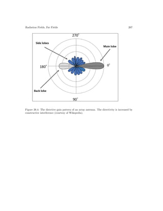
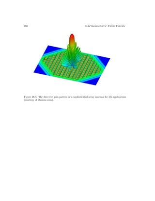
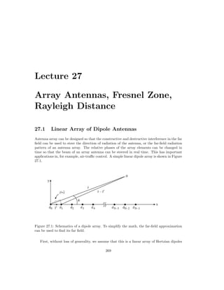
![270 Electromagnetic Field Theory
aligned on the x axis. The current can then be described mathematically as follows:
J(r0
) = ẑIl[A0δ(x0
) + A1δ(x0
− d1) + A2δ(x0
− d2) + · · ·
+ AN−1δ(x0
− dN−1)]δ(y0
)δ(z0
) (27.1.1)
27.1.1 Far-Field Approximation
The vector potential on the xy-plane in the far field, using the sifting property of delta
function, yield the following equation, to be
A(r) ∼
= ẑ
µIl
4πr
e−jβr
dr0
[A0δ(x0
) + A1δ(x0
− d1) + · · · ]δ(y0
)δ(z0
)ejβr0
·r̂
= ẑ
µIl
4πr
e−jβr
[A0 + A1ejβd1 cos φ
+ A2ejβd2 cos φ
+ · · · + AN−1ejβdN−1 cos φ
] (27.1.2)
In the above, we have assumed that the observation point is on the xy plane, or that r = ρ =
x̂x + ŷy. Thus, r̂ = x̂ cos φ + ŷ sin φ. Also, since the sources are aligned on the x axis, then
r0
= x̂x0
, and r0
· r̂ = x0
cos φ. Consequently, ejβr0
·r̂
= ejβx0
cos φ
.
If dn = nd, and An = ejnψ
, then the antenna array, which assumes a progressively
increasing phase shift between different elements, is called a linear phase array. Thus, (27.1.2)
in the above becomes
A(r) ∼
= ẑ
µIl
4πr
e−jβr
[1 + ej(βd cos φ+ψ)
+ ej2(βd cos φ+ψ)
+ · · ·
+ej(N−1)(βd cos φ+ψ)
] (27.1.3)
27.1.2 Radiation Pattern of an Array
The above(27.1.3) can be summed in closed form using
N−1
X
n=0
xn
=
1 − xN
1 − x
(27.1.4)
Then in the far field,
A(r) ∼
= ẑ
µIl
4πr
e−jβr 1 − ejN(βd cos φ+ψ)
1 − ej(βd cos φ+ψ)
(27.1.5)
Ordinarily, as shown previously, E ≈ −jω(θ̂Aθ + φ̂Aφ). But since A is ẑ directed, Aφ = 0.
Furthermore, on the xy plane, Eθ ≈ −jωAθ = jωAz. Therefore,
|Eθ| = |E0|
1 − ejN(βd cos φ+ψ)
1 − ej(βd cos φ+ψ)
, r → ∞
= |E0|
sin N
2 (βd cos φ + ψ)
sin 1
2 (βd cos φ + ψ)
, r → ∞ (27.1.6)](https://image.slidesharecdn.com/emftall20191204-240115133321-d13ecad1/85/EMFTAll2-284-320.jpg)
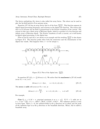
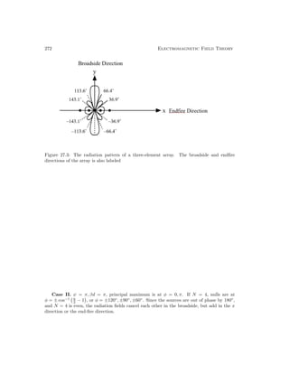
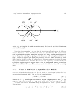
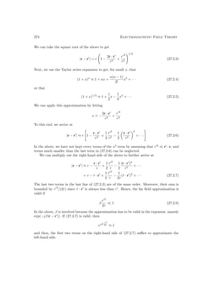
![Array Antennas, Fresnel Zone, Rayleigh Distance 275
27.2.1 Rayleigh Distance
Figure 27.5: The right half of a Gaussian beam [74] displays the physics of the near field, the
Fresnel zone, and the far zone. In the far zone, the field behaves like a spherical wave.
When a wave field leaves an aperture antenna, it can be approximately described by a Gaus-
sian beam [74] (see Figure 27.5). Near to the antenna aperture, or the near zone, it is
approximately a plane wave with wave fronts parallel to the aperture surface. Far from the
antenna aperture, or in the far zone, the field behaves like a spherical wave, with its typical
wave front. In between is the Fresnel zone.
Consequently, after using that β = 2π/λ, for the far-field approximation to be valid, we
need (27.2.8), or that
r
π
λ
r2
(27.2.9)
If the aperture of the antenna is of radius W, then r
rmax
∼
= W and the far field approxi-
mation is valid if
r
π
λ
W2
= rR (27.2.10)
If r is larger than this distance, then an antenna beam behaves like a spherical wave and starts
to diverge. This distance rR is also known as the Rayleigh distance. After this distance, the
wave from a finite size source resembles a spherical wave which is diverging in all directions.
Also, notice that the shorter the wavelength λ, the larger is this distance. This also explains
why a laser pointer works. A laser pointer light can be thought of radiation from a finite size
source located at the aperture of the laser pointer. The laser pointer beam remains collimated
for quite a distance, before it becomes a divergent beam or a beam with a spherical wave
front.](https://image.slidesharecdn.com/emftall20191204-240115133321-d13ecad1/85/EMFTAll2-289-320.jpg)
![276 Electromagnetic Field Theory
In some textbooks [31], it is common to define acceptable phase error to be π/8. The
Rayleigh distance is the distance beyond which the phase error is below this value. When the
phase error of π/8 is put on the right-hand side of (27.2.8), one gets
β
r02
2r
≈
π
8
(27.2.11)
Using the approximation, the Rayleigh distance is defined to be
rR =
2D2
λ
(27.2.12)
where D = 2W is the diameter of the antenna aperture.
27.2.2 Near Zone, Fresnel Zone, and Far Zone
Therefore, when a source radiates, the radiation field is divided into the near zone, the Fresnel
zone, and the far zone (also known as the radiation zone, or the Fraunhofer zone in optics).
The Rayleigh distance is the demarcation boundary between the Fresnel zone and the far
zone. The larger the aperture of an antenna array is, the further one has to be to reach the
far zone of an antenna. This distance becomes larger too when the wavelength is short. In the
far zone, the far field behaves like a spherical wave, and its radiation pattern is proportional
to the Fourier transform of the current.
In some sources, like the Hertzian dipole, in the near zone, much reactive energy is stored
in the electric field or the magnetic field near to the source. This near zone receives reactive
power from the source, which corresponds to instantaneous power that flows from the source,
but is return to the source after one time harmonic cycle. Hence, a Hertzian dipole has input
impedance that looks like that of a capacitor, because much of the near field of this dipole is
in the electric field.
The field in the far zone carries power that radiates to infinity. As a result, the field in the
near zone decays rapidly, but the field in the far zone decays as 1/r for energy conservation.](https://image.slidesharecdn.com/emftall20191204-240115133321-d13ecad1/85/EMFTAll2-290-320.jpg)
![Lecture 28
Different Types of
Antennas–Heuristics
28.1 Types of Antennas
There are different types of antennas for different applications [127]. We will discuss their
functions heuristically in the following discussions.
28.1.1 Resonance Tunneling in Antenna
A simple antenna like a short dipole behaves like a Hertzian dipole with an effective length.
A short dipole has an input impedance resembling that of a capacitor. Hence, it is difficult
to drive current into the antenna unless other elements are added. Hertz used two metallic
spheres to increase the current flow. When a large current flows on the stem of the Hertzian
dipole, the stem starts to act like inductor. Thus, the end cap capacitances and the stem
inductance together can act like a resonator enhancing the current flow on the antenna.
Some antennas are deliberately built to resonate with its structure to enhance its radiation.
A half-wave dipole is such an antenna as shown in Figure 28.1 [123]. One can think that these
antennas are using resonance tunneling to enhance their radiation efficiencies. A half-wave
dipole can also be thought of as a flared open transmission line in order to make it radiate.
It can be gradually morphed from a quarter-wavelength transmission line as shown in Figure
28.1. A transmission is a poor radiator, because the electromagnetic energy is trapped between
two pieces of metal. But a flared transmission line can radiate its field to free space. The
dipole antenna, though a simple device, has been extensively studied by King [128]. He has
reputed to have produced over 100 PhD students studying the dipole antenna.
277](https://image.slidesharecdn.com/emftall20191204-240115133321-d13ecad1/85/EMFTAll2-291-320.jpg)
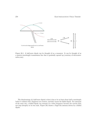
![Different Types of Antennas–Heuristics 279
Figure 28.2: In a Yagi-Uda antenna, when a wire antenna is less than half a wavelength,
it acts as a waveguide, or a director. Then the wire antenna is slightly more than half a
wavelength, it acts as a reflector [129]. Therefore, the antenna radiates predominantly in one
direction (courtesy of Wikipedia [130]).
A Yagi-Uda antenna is also another interesting invention. It was invented in 1926 by
Yagi and Uda in Japan by plainly using physical intuition [129]. Physical intuition was a
tool of engineers of yesteryears while modern engineers tend to use sophisticated computer
design software. Surprisingly, the elements of dipoles in front of the driver element are acting
like a waveguide in space, while the element at the back acts like a reflector. Therefore, the
field radiated by the driver element will be directed toward the front of the antenna. Thus,
this antenna has higher directivity than just a stand alone dipole. Due to its simplicity, this
antenna has been made into nano-antennas which can radiate at optical frequencies.](https://image.slidesharecdn.com/emftall20191204-240115133321-d13ecad1/85/EMFTAll2-293-320.jpg)
![280 Electromagnetic Field Theory
Figure 28.3: A cavity-backed slot antenna radiates well because when the small dipole radiates
close to the resonant frequency of the cavity, the field strength is strong inside the cavity, and
hence around the slot (courtesy of antenna-theory.com).
Slot antenna is a simple antenna to make [131]. To improve the radiation efficiency of
slot antenna, it is made to radiate via a cavity. A cavity-backed slot antenna that uses such
a concept and this is shown in Figure 28.3. A small dipole with poor radiation efficiency is
places inside the cavity. When the operating frequency is close to the resonant frequency of
the cavity, the field strength inside the cavity becomes strong, and much of the energy can
leak from the cavity via the slot on its side. This makes the antenna radiate more efficiently
into free space compared to just the small dipole alone.
Another antenna that resembles a cavity backed slot antenna is the patch antenna, or
microstrip patch antenna. This is shown in in Figure 28.4. This antenna also radiates
efficiently by resonant tunneling. The resonant frequency of the patch antenna (top of Figure
28.4) is roughly when L is half a wavelength. This is similar to the resonant frequency of a
transmission line with open circuit at both ends. The current sloshes back and forth across
the length of the patch antenna along the L direction. The second design (bottom of Figure
28.4) has an inset feed. This allows the antenna to resonate at a lower frequency because the
current has a longer path to slosh through when it is at resonance.](https://image.slidesharecdn.com/emftall20191204-240115133321-d13ecad1/85/EMFTAll2-294-320.jpg)
![Different Types of Antennas–Heuristics 281
Figure 28.4: A patch antenna also radiates well when it resonates. The patch antenna
resembles a cavity resonator with magnetic wall (courtesy of emtalk.com).
28.1.2 Horn Antennas
The impedance of space is 377 ohms while that of most transmission line is 50 ohms. This
mismatch can be mitigated by using a flared horn (see Figure 28.5) [132].
One can think that the characteristic impedance of a transmission line made of two pieces
of metal as Z0 =
L/C. As the horn flares, C becomes smaller, increasing its characteristic
impedance to get close to that of free space. This allows for better impedance matching from
the source to free space.
A corrugated horn, as we have discussed previously in a circular waveguide, discourages
current flows in the non-axial symmetric mode. It encourages the propagation of the TE01
mode in the circular waveguide and hence, the circular horn antenna. This mode is axially
symmetric. Hence, this antenna can radiate fields that are axially symmetric [133,134].](https://image.slidesharecdn.com/emftall20191204-240115133321-d13ecad1/85/EMFTAll2-295-320.jpg)
![282 Electromagnetic Field Theory
Figure 28.5: A horn antenna works with the same principle as the biconical antenna. Its
flared horn changes the waveguide impedance so as to match from that of a waveguide to
that of free space. The lower figure is that of a corrugated circular horn antenna. The
corrugation enhances the propagation of the TE01 mode in the circular waveguide, and hence,
the cylindrical symmetry of the mode (courtesy of tutorialpoints.com and comsol.com).
A Vivaldi antenna (invented by P. Gibson in 1978 [135]), is shown in Figure 28.6. It is also
called a notch antenna. It works by the same principle to gradually match the impedance of
the source to that of free space. But such a gradually flared horn has the element of a frequency
independent antenna. The low frequency component of the signal will radiate from the wide
end of the flared notch, while the high frequency component will radiate from the narrow end
of the notch. Thus, this antenna can radiate well over a broad range of frequencies, and this
gives the antenna a broad bandwidth performance. It is good for transmitting a pulsed signal
which has a broad frequency spectrum.](https://image.slidesharecdn.com/emftall20191204-240115133321-d13ecad1/85/EMFTAll2-296-320.jpg)
![Different Types of Antennas–Heuristics 283
Figure 28.6: A Vivaldi antenna works iike a horn antenna, but uses very little metal. Hence,
it is cheap to build (courtesy of Wikipedia [136]).
28.1.3 Quasi-Optical Antennas
High-frequency or short wavelength electromagnetic field behaves like light ray as in optics.
Therefore, many high-frequency antennas are designed based on the principle of ray optics.
A reflector antenna is such an antenna as shown in Figure 28.7. The reflector antenna in this
case is a Cassegrain design [137]1
where a sub-reflector is present. This allows the antenna
to be fed from behind the parabolic dish where the electronics can be stored and isolated as
well. Reflector antennas [139] is used a lot in radio astronomy and space exploration due to
their high directivity and sensitivity.
1The name came from an optical telescope of similar design [138]](https://image.slidesharecdn.com/emftall20191204-240115133321-d13ecad1/85/EMFTAll2-297-320.jpg)
![284 Electromagnetic Field Theory
Figure 28.7: The top picture of an NRAO radio telescope antenna of Cassegrain design
(courtesy of Britannica.com). The bottom is the detail of the Cassegrain design (courtesy of
rev.com).
Another recent invention is the reflectarray antenna [140,141] which is very popular. One
of them is as shown in Figure 28.8. Due to recent advent in simulation technology, complicated
structures can be simulated on a computer, including one with a complicated surface design.
Patch elements can be etched onto a flat surface as shown, giving it effective impedance that
is spatially varying, making it reflect like a curved surface. Such a surface is known as a
meta-surface [142,143]. It can greatly economize on the space of a reflector antenna.](https://image.slidesharecdn.com/emftall20191204-240115133321-d13ecad1/85/EMFTAll2-298-320.jpg)
![Different Types of Antennas–Heuristics 285
Figure 28.8: A reflectarray where the reflector is a flat surface. Patches are unequally spaced
to give the array the focussing effect (courtesy of antenna-theory.com).
Another quasi-optical antenna is the lens antenna as shown in Figure 28.9 [144]. The
design of this antenna follows lens optics, and is only valid when the wavelength is very short
compared to the curvature of the surfaces. In this case, reflection and transmission at a curve
surface is similar to that of a flat surface. This is called the tangent-plane approximation of
a curve surface, and is valid at high frequencies.](https://image.slidesharecdn.com/emftall20191204-240115133321-d13ecad1/85/EMFTAll2-299-320.jpg)
![286 Electromagnetic Field Theory
Figure 28.9: The top figure shows a lens antenna where the lens is made of artificial dielectrics
made from metallic strips (courtesy of electriciantutoring.tpub.com). The bottom figure shows
some dielectric lens at the aperture of an open waveguide to focus the microwave exiting from
the waveguide opening (courtesy of micro-radar.de).
28.1.4 Small Antennas
Small antennas are in vogue these days due to the advent of the cell phone, and the importance
of economizing on the antenna size. Also, the antennas should have enough bandwidth to
accommodate the signals from different cell phone companies, which use different carrier
frequencies. An interesting small antenna is the PIFA (planar inverted F antenna) shown in
Figure 28.10 [145]. Because it is shorted at one end and open circuit at the other end, it acts
like a quarter wavelength resonator, making it substantially smaller. But the resonator is low
Q because of the “slots” around it from whom energy can leak. The low Q gives this antenna
a broader bandwidth.](https://image.slidesharecdn.com/emftall20191204-240115133321-d13ecad1/85/EMFTAll2-300-320.jpg)
![Different Types of Antennas–Heuristics 287
Figure 28.10: A PIFA (planar inverted F antenna) is compact, broadband, and easy to
fabricate. It is good for cell phone antennas due to its small size (courtesy of Mathworks).
An interesting small antenna is the U-slot antenna shown in Figure 28.11 [146,147]. Be-
cause the current is forced to follow a longer path by the U-slot, it has a lower resonant
frequency and hence, can be made smaller. In order to give the antenna a larger bandwidth,
its Q is made smaller by etching it on a thick dielectric substrate (shown as the dielectric
material region in the figure). But feeding it with a longer probe will make the bandwidth
of the antenna smaller, due to the larger inductance of the probe. An ingenious invention
is to use an L probe [148]. The L probe has an inductive part as well as a capacitive part.
Their reactance cancel each other, allowing the electromagnetic energy to tunnel through the
antenna, making it a better radiator.](https://image.slidesharecdn.com/emftall20191204-240115133321-d13ecad1/85/EMFTAll2-301-320.jpg)
![288 Electromagnetic Field Theory
Figure 28.11: The top figure shows a U slot patch antenna design. The bottom figure shows
a patch antenna fed by an L probe with significant increase in bandwidth (courtesy of K.M.
Luk) [148].
Another area where small antennas are needed is in RFID (radio frequency identification)
tag [149]. Since tags are placed outside the packages of products, an RFID tag has a transmit-
receive antenna which can talk to a small computer chip where data about the package can be
stored. An RFID reader can quickly communicate with the RFID tag to retrieve information
about the package. Such a small antenna design for RFID tag is shown in Figure 28.12. It
uses image theorem so that the antenna can be made half as small. Then slots are cut into the
radiating patch, so that the current follows a longer path. This lowers the resonant frequency
of the antenna, allowing it to be made smaller.](https://image.slidesharecdn.com/emftall20191204-240115133321-d13ecad1/85/EMFTAll2-302-320.jpg)
![Different Types of Antennas–Heuristics 289
Figure 28.12: Some RFID antennas designed at The University of Hong Kong (courtesy of P.
Yang, Y. Li, J. Huang, L.J. Jiang, S.Q. He, T. Ye, and W.C. Chew).
An RFID reader can be designed to read the information from a batch of vials or tubes
containing different chemicals. Hence, a large loop antenna is needed at a sufficiently high
frequency (for large bandwidth). However, driving a loop antenna at a sufficiently high
frequency will result in a non-constant current around the loop. (Fundamentally, this comes
from the retardation effect of electromagnetic field.) This will result in a non-uniform field
inside the loop defeating the design of the RFID reader.
One way to view how the non-uniform current come about is that a piece of wire becomes
a tiny inductor. Across an inductor, V = jωLI, implying a 90◦
phase shift between the
voltage and the current. In other words, the voltage drop is always nonzero, and hence, the
voltage cannot be constant around the loop. Since the voltage and current are locally related
by the local inductance, the current cannot be constant also.
To solve the problem of the current and voltage being non-constant around the loop, the
local inductor is connected in series with a capacitor [150]. This causes them to resonate.
At resonance, the current-voltage relationship across the tank circuit is such that there is no
voltage drop across the tank circuit. In this case, the voltage becomes uniform across the
loop so is the current. Therefore, one way to enable a uniform current in a large loop is
to capacitively load the loop. This will ensure a constant phase, or a more uniform current
around the loop, and hence, a more efficient reader. Such a design is shown in Figure 28.13.](https://image.slidesharecdn.com/emftall20191204-240115133321-d13ecad1/85/EMFTAll2-303-320.jpg)
![290 Electromagnetic Field Theory
Figure 28.13: The top figure shows a RFID reader designed by [151]. The bottom figure
shows simulation and measurement done at The University of Hong Kong (courtesy of Z.N.
Chen [151] and P. Yang, Y. Li, J. Huang, L.J. Jiang, S.Q. He, T. Ye, and W.C. Chew).](https://image.slidesharecdn.com/emftall20191204-240115133321-d13ecad1/85/EMFTAll2-304-320.jpg)
![Lecture 29
Uniqueness Theorem
29.1 Uniqueness Theorem
The uniqueness of a solution to a linear system of equations is an important concept in
mathematics. Under certain conditions, ordinary differential equation partial differential
equation and matrix equations will have unique solutions. But uniqueness is not always
guaranteed as we shall see. This issue is discussed in many math books and linear algebra
books [69, 81]. The prove of uniqueness for Laplace and Poisson equations are given in
[29,48] which is slightly different for electrodynamic problems. In this section, we will prove
uniqueness theorem for electrodynamic problems [31,34,47,59,75]. First, let us assume that
there exist two solutions in the presence of one set of common impressed sources Ji and Mi.
Namely, these two solutions are Ea
, Ha
, Eb
, Hb
. Both of them satisfy Maxwell’s equations
and the same boundary conditions. Are Ea
= Eb
, Ha
= Hb
?
To study the uniqueness theorem, we consider general linear anisotropic inhomogeneous
media, where the tensors µ and ε can be complex so that lossy media can be included, it
follows that
∇ × Ea
= −jωµ · Ha
− Mi (29.1.1)
∇ × Eb
= −jωµ · Hb
− Mi (29.1.2)
∇ × Ha
= jωε · Ea
+ Ji (29.1.3)
∇ × Hb
= jωε · Eb
+ Ji (29.1.4)
By taking the difference of these two solutions, we have
∇ × (Ea
− Eb
) = −jωµ · (Ha
− Hb
) (29.1.5)
∇ × (Ha
− Hb
) = jωε · (Ea
− Eb
) (29.1.6)
Or alternatively, defining δE = Ea
− Eb
and δH = Ha
− Hb
, we have
∇ × δE = −jωµ · δH (29.1.7)
∇ × δH = jωε · δE (29.1.8)
291](https://image.slidesharecdn.com/emftall20191204-240115133321-d13ecad1/85/EMFTAll2-305-320.jpg)
![292 Electromagnetic Field Theory
The difference solutions satisfy the original source-free Maxwell’s equations.
By taking the left dot product of δH∗
with (29.1.7), and then the left dot product of δE∗
with the complex conjugation of (29.1.8), we obtain
δH∗
· ∇ × δE = −jωδH∗
· µ · δH
δE · ∇ × δH∗
= −jωδE · ε∗
· δE∗
(29.1.9)
Now, taking the difference of the above, we get
δH∗
· ∇ × δE − δE · ∇ × δH∗
= ∇ · (δE × δH∗
)
= −jωδH∗
· µ · δH + jωδE · ε∗
· δE∗
(29.1.10)
Figure 29.1: Geometry for proving the uniqueness theorem. We like to know the boundary
conditions needed on S in order to guarantee the uniqueness of the solution in V .
Next, integrating the above equation over a volume V bounded by a surface S as shown
in Figure 29.1. Two scenarios are possible: one that the volume V contains the impressed
sources, and two, that the sources are outside the volume V . After making use of Gauss’
divergence theorem, we arrive at
V
∇ · (δE × δH∗
)dV =
S
(δE × δH∗
) · dS
=
V
[−jωδH∗
· µ · δH + jωδE · ε∗
· δE∗
]dV (29.1.11)
And next, we would like to know the kind of boundary conditions that would make the
left-hand side equal to zero. It is seen that the surface integral on the left-hand side will be](https://image.slidesharecdn.com/emftall20191204-240115133321-d13ecad1/85/EMFTAll2-306-320.jpg)
![Uniqueness Theorem 293
zero if:1
1. If n̂×E is specified over S so that n̂×Ea = n̂×Eb, then n̂×δE = 0 or the PEC boundary
condition for δE, and then2
S
(δE × δH∗
) · n̂dS = S
(n̂ × δE) · δH∗
dS = 0.
2. If n̂ × H is specified over S so that n̂ × Ha = n̂ × Hb, then n̂ × δH = 0 or the PMC
boundary condition for δH, and then
S
(δE × δH∗
) · n̂dS = − S
(n̂ × δH∗
) · δEdS = 0.
3. If n̂ × E is specified over S1, and n̂ × H is specified over S2 (where S1 ∪ S2 = S), then
n̂ × δE = 0 (PEC boundary condition) on S1, and n̂ × δH = 0 (PMC boundary condition)
on S2, then the left-hand side becomes
S
(δE × δH∗
) · n̂dS =
S1
+
S2
=
S1
(n̂ × δE) · δH∗
dS
−
S2
(n̂ × δH∗
) · δEdS = 0.
Thus, under the above three scenarios, the left-hand side of (29.1.11) is zero, and then
the right-hand side of (29.1.11) becomes
V
[−jωδH∗
· µ · δH + jωδE · ε∗
· δE∗
]dV = 0 (29.1.12)
For lossless media, µ and ε are hermitian tensors (or matrices3
), then it can be seen, using
the properties of hermitian matrices or tensors, that δH∗
· µ · δH and δE · ε∗
· δE∗
are purely
real. Taking the imaginary part of the above equation yields
V
[−δH∗
· µ · δH + δE · ε∗
· δE∗
]dV = 0 (29.1.13)
The above two terms correspond to stored magnetic field energy and stored electric field
energy in the difference solutions δH and δE, respectively. The above being zero does not
imply that δH and δE are zero.
For resonance solutions, the stored electric energy can balance the stored magnetic energy.
The above resonance solutions are those of the difference solutions satisfying PEC or PMC
boundary condition or mixture thereof. Therefore, δH and δE need not be zero, even though
(29.1.13) is zero. This happens when we encounter solutions that are the resonant modes of
the volume V bounded by surface S.
Uniqueness can only be guaranteed if the medium is lossy as shall be shown later. It is
also guaranteed if lossy impedance boundary conditions are imposed.4
First we begin with
the isotropic case.
1In the following, please be reminded that PEC stands for “perfect electric conductor”, while PMC stands
for “perfect magnetic conductor”. PMC is the dual of PEC. Also, a fourth case of impedance boundary
condition is possible, which is beyond the scope of this course. Interested readers may consult Chew, Theory
of Microwave and Optical Waveguides [75].
2Using the vector identity that a · (b × c) = c · (a × b) = b · (c × a).
3Tensors are a special kind of matrices.
4See Chew, Theory of Microwave and Optical Waveguides.](https://image.slidesharecdn.com/emftall20191204-240115133321-d13ecad1/85/EMFTAll2-307-320.jpg)
![294 Electromagnetic Field Theory
29.1.1 Isotropic Case
It is easier to see this for lossy isotropic media. Then (29.1.12) simplifies to
V
[−jωµ|δH|2
+ jωε∗
|δE|2
]dV = 0 (29.1.14)
For isotropic lossy media, µ = µ0
− jµ00
and ε = ε0
− jε00
. Taking the real part of the above,
we have from (29.1.14) that
V
[−ωµ00
|δH|2
− ωε00
|δE|2
]dV = 0 (29.1.15)
Since the integrand in the above is always negative definite, the integral can be zero only if
δE = 0, δH = 0 (29.1.16)
everywhere in V , implying that Ea = Eb, and that Ha = Hb. Hence, it is seen that uniqueness
is guaranteed only if the medium is lossy. The physical reason is that when the medium is
lossy, a pure time-harmonic solution cannot exist due to loss. The modes, which are the
source-free solutions of Maxwell’s equations, are decaying sinusoids.
Notice that the same conclusion can be drawn if we make µ00
and ε00
negative. This
corresponds to active media, and uniqueness can be guaranteed for a time-harmonic solution.
In this case, no time-harmonic solution exists, and the resonant solution is a growing sinusoid.
29.1.2 General Anisotropic Case
The proof for general anisotropic media is more complicated. For the lossless anisotropic
media, we see that (29.1.12) is purely imaginary. However, when the medium is lossy, this
same equation will have a real part. Hence, we need to find the real part of (29.1.12) for the
general lossy case.
About taking the Real and Imaginary Parts of a Complex Expression
To this end, we digress on taking the real and imaginary parts of a complex expression. Here,
we need to find the complex conjugate5
of (29.1.12), which is scalar, and add it to itself to
get its real part. The complex conjugate of the scalar
c = δH∗
· µ · δH
is6
c∗
= δH · µ∗
· δH∗
= δH∗
· µ†
· δH
5Also called hermitian conjugate.
6To arrive at these expressions, one makes use of the matrix algebra rule that if D = A · B · C, then
D
t
= C
t
· B
t
· A
t
. This is true even for non-square matrices. But for our case here, A is a 1 × 3 row vector,
and C is a 3×1 column vector, and B is a 3×3 matrix. In vector algebra, the transpose of a vector is implied.
Also, in our case here, D is a scalar, and hence, its transpose is itself.](https://image.slidesharecdn.com/emftall20191204-240115133321-d13ecad1/85/EMFTAll2-308-320.jpg)
![Uniqueness Theorem 295
Similarly, the complex conjugate of the scalar
d = δE · ε∗
· δE∗
= δE∗
· ε†
· δE
is
d∗
= δE∗
· ε†
· δE
Therefore,
=m (δH∗
· µ · δH) =
1
2j
δH∗
· (µ − µ†
) · δH
=m (δE · ε · δE∗
) =
1
2j
δE∗
· (ε − ε†
) · δE
and similarly for the real part.
Finally, after taking the complex conjugate of the scalar quantity (29.1.12) and adding it
to itself, we have
V
[−jωδH∗
· (µ − µ†
) · δH − jωδE∗
· (ε − ε†
) · δE]dV = 0 (29.1.17)
For lossy media, −j(µ − µ†
) and −j(ε − ε†
) are hermitian negative matrices. Hence the
integrand is always negative definite, and the above equation cannot be satisfied unless δH =
δE = 0 everywhere in V . Thus, uniqueness is guaranteed in a lossy anisotropic medium.
Similar statement can be made as the isotropic case if the medium is active. Then the
integrand is positive definite, and the above equation cannot be satisfied unless δH = δE = 0
everywhere in V and hence, uniqueness is satisfied.
29.1.3 Hind Sight
The proof of uniqueness for Maxwell’s equations is very similar to the proof of uniqueness for
a matrix equation [69]
A · x = b (29.1.18)
If a solution to a matrix equation exists without excitation, namely, when b = 0, then the
solution is the null space solution [69], namely, x = xN . In other words,
A · xN = 0 (29.1.19)
These null space solutions exist without a “driving term” b on the right-hand side. For
Maxwell’s Equations, b corresponds to the source terms. They are like the homogeneous
solution of an ordinary differential equation or a partial differential equation [81]. In an
enclosed region of volume V bounded by a surface S, homogeneous solutions are the resonant
solutions of this Maxwellian system. When these solutions exist, they give rise to non-
uniqueness.
Also, notice that (29.1.7) and (29.1.8) are Maxwell’s equations without the source terms.
In a closed region V bounded by a surface S, only resonance solutions for δE and δH with
the relevant boundary conditions can exist when there are no source terms.](https://image.slidesharecdn.com/emftall20191204-240115133321-d13ecad1/85/EMFTAll2-309-320.jpg)
![296 Electromagnetic Field Theory
As previoulsy mentioned, one way to ensure that these resonant solutions are eliminated
is to put in loss or gain. When loss or gain is present, then the resonant solutions are decaying
sinusoids or growing sinusoids. Since we are looking for solutions in the frequency domain,
or time harmonic solutions, we are only looking for the solution on the real ω axis on the
complex ω plane. These non-sinusoidal solutions are outside the solution space: They are
not part of the time-harmonic solutions we are looking for. Therefore, there are no resonant
null-space solutions.
29.1.4 Connection to Poles of a Linear System
The output to input of a linear system can be represented by a transfer function H(ω) [45,152].
If H(ω) has poles, and if the system is lossless, the poles are on the real axis. Therefore, when
ω = ωpole, the function H(ω) becomes undefined. This also gives rise to non-uniqueness of the
output with respect to the input. Poles usually correspond to resonant solutions, and hence,
the non-uniqueness of the solution is intimately related to the non-uniqueness of Maxwell’s
equations at the resonant frequencies of a structure. This is illustrated in the upper part of
Figure 29.2.
Figure 29.2: The non-uniqueness problem is intimately related to the locations of the poles
of a transfer function being on the real axis.](https://image.slidesharecdn.com/emftall20191204-240115133321-d13ecad1/85/EMFTAll2-310-320.jpg)
![Uniqueness Theorem 297
If the input function is f(t), with Fourier transform F(ω), then the output y(t) is given
by the following Fourier integral, viz.,
y(t) =
1
2π
∞
−∞
dωejωt
H(ω)F(ω) (29.1.20)
where the Fourier inversion integral path is on the real axis on the complex ω plane. The
Fourier inversion integral is undefined or non-unique.
However, if loss is introduced, these poles will move away from the real axis as shown
in the lower part of Figure 29.2. Then the transfer function is uniquely determined for all
frequencies on the real axis. In this way, the Fourier inversion integral in (29.1.20) is well
defined, and uniqueness of the solution is guaranteed.
29.1.5 Radiation from Antenna Sources
The above uniqueness theorem guarantees that if we have some antennas with prescribed
current sources on them, the radiated field from these antennas are unique. To see how this
can come about, we first study the radiation of sources into a region V bounded by a large
surface Sinf as shown in Figure 29.3 [34].
Even when n̂ × E or n̂ × H are specified on the surface at Sinf, the solution is nonunique
because the volume V bounded by Sinf, can have many resonant solutions. In fact, the
region will be replete with resonant solutions as one makes Sinf become very large. The way
to remove these resonant solutions is to introduce an infinitesimal amount of loss in region
V . Then these resonant solutions will disappear. Now we can take Sinf to infinity, and the
solution will always be unique.
Notice that if Sinf → ∞, the waves that leave the sources will never be reflected back
because of the small amount of loss. The radiated field will just disappear into infinity. This
is just what radiation loss is: power that propagate to infinity, but never to return. In fact,
one way of guaranteeing the uniqueness of the solution in region V when Sinf is infinitely large,
or that V is infinitely large is to impose the radiation condition: the waves that radiate to
infinity are outgoing waves only, and never do they return. This is also called the Sommerfeld
radiation condition [153]. Uniqueness of the field outside the sources is always guaranteed if
we assume that the field radiates to infinity and never to return. This is equivalent to solving
the cavity solutions with an infinitesimal loss, and then letting the size of the cavity become
infinitely large.](https://image.slidesharecdn.com/emftall20191204-240115133321-d13ecad1/85/EMFTAll2-311-320.jpg)
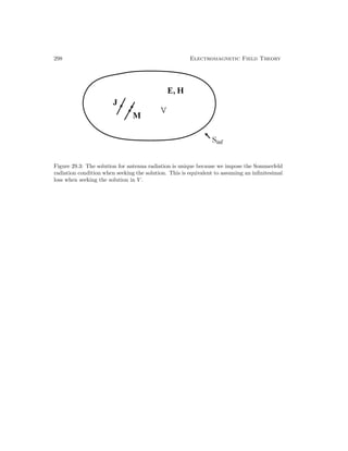
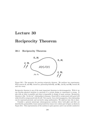
![300 Electromagnetic Field Theory
media as well. It can represent complex terrain as well as complicated electronic circuit
structures in circuit boards or microchips, and complicated antenna structures.
When only J1 and M1 are turned on, they generate fields E1 and H1 in this medium.
On the other hand, when only J2 and M2 are turned on, they generate E2 and H2 in this
medium. Therefore, the pertinent equations, for linear time-invariant systems, for these two
cases are1
∇ × E1 = −jωµ · H1 − M1 (30.1.1)
∇ × H1 = jωε · E1 + J1 (30.1.2)
∇ × E2 = −jωµ · H2 − M2 (30.1.3)
∇ × H2 = jωε · E2 + J2 (30.1.4)
From the above, we can show that (after left dot-multiply (30.1.1) with H2 and (30.1.4) with
E1),
H2 · ∇ × E1 = −jωH2 · µ · H1 − H2 · M1 (30.1.5)
E1 · ∇ × H2 = jωE1 · ε · E2 + E1 · J2 (30.1.6)
Then, using the above, and the following identity, we get the second equality in the following
expression:
∇ · (E1 × H2) = H2 · ∇ × E1 − E1 · ∇ · H2
= −jωH2 · µ · H1 − jωE1 · ε · E2 − H2 · M1 − E1 · J2 (30.1.7)
By the same token,
∇ · (E2 × H1) = −jωH1 · µ · H2 − jωE2 · ε · E1 − H1 · M2 − E2 · J1 (30.1.8)
If one assumes that
µ = µt
, ε = εt
(30.1.9)
or when the tensors are symmetric, then H1 ·µ·H2 = H2 ·µ·H1 and E1 ·ε·E2 = E2 ·ε·E1.2
Upon subtracting (30.1.7) and (30.1.8), one gets
∇ · (E1 × H2 − E2 × H1) = −H2 · M1 − E1 · J2 + H1 · M2 + E2 · J1 (30.1.10)
1The current sources are impressed currents so that they are immutable, and not changed by the environ-
ment they are immersed in [47].
2It is to be noted that in matrix algebra, the dot product between two vectors are often written as at · b,
but in the physics literature, the transpose on a is implied. Therefore, the dot product between two vectors
is just written as a · b.](https://image.slidesharecdn.com/emftall20191204-240115133321-d13ecad1/85/EMFTAll2-314-320.jpg)
![Reciprocity Theorem 301
Figure 30.2: The geometry for proving reciprocity theorem when the surface S does not
enclose the sources.
Figure 30.3: The geometry for proving reciprocity theorem when the surface S encloses the
sources.
Now, integrating (30.1.10) over a volume V bounded by a surface S, and invoking Gauss’
divergence theorem, we have the reciprocity theorem that
S
dS · (E1 × H2 − E2 × H1)
= −
V
dV [H2 · M1 + E1 · J2 − H1 · M2 − E2 · J1] (30.1.11)
When the volume V contains no sources (see Figure 30.2), the reciprocity theorem reduces to
S
dS · (E1 × H2 − E2 × H1) = 0 (30.1.12)
The above is also called Lorentz reciprocity theorem by some authors.3
Next, when the surface S contains all the sources (see Figure 30.3), then the right-hand
side of (30.1.11) will not be zero. On the other hand, when the surface S → ∞, E1 and
3Harrington, Time-Harmonic Electric Field [47].](https://image.slidesharecdn.com/emftall20191204-240115133321-d13ecad1/85/EMFTAll2-315-320.jpg)
![302 Electromagnetic Field Theory
H2 becomes spherical waves which can be approximated by plane waves sharing the same β
vector. Moreover, under the plane-wave approximation, ωµ0H2 = β × E2, ωµ0H1 = β × E1,
then
E1 × H2 ∼ E1 × (β × E2) = E1(β · E2) − β(E1 · E2) (30.1.13)
E2 × H1 ∼ E2 × (β × E1) = E2(β · E1) − β(E2 · E1) (30.1.14)
But β ·E2 = β ·E1 = 0 in the far field and the β vectors are parallel to each other. Therefore,
the two terms on the left-hand side of (30.1.11) cancel each other, and it vanishes when
S → ∞. (Furthermore, they cancel each other so that the remnant field vanishes faster than
1/r2
. This is necessary as the surface area S is growing larger and proportional to r2
.)
As a result, (30.1.11) can be rewritten simply as
V
dV [E2 · J1 − H2 · M1] =
V
dV [E1 · J2 − H1 · M2] (30.1.15)
The inner product symbol is often used to rewrite the above as
hE2, J1i − hH2, M1i = hE1, J2i − hH1, M2i (30.1.16)
where the inner product hA, Bi =
V
dV A(r) · B(r).
The above inner product is also called reaction, a concept introduced by Rumsey. There-
fore, the above is rewritten more succinctly as
h2, 1i = h1, 2i (30.1.17)
where
h2, 1i = hE2, J1i − hH2, M1i (30.1.18)
The concept of inner product or reaction can be thought of as a kind of “measurement”. The
reciprocity theorem can be stated as that the fields generated by sources 2 as “measured”
by sources 1 is equal to fields generated by sources 1 as “measured” by sources 2. This
measurement concept is more lucid if we think of these sources as Hertzian dipoles.
30.1.1 Conditions for Reciprocity
It is seen that the above proof hinges on (30.1.9). In other words, the anisotropic medium has
to be described by symmetric tensors. They include conductive media, but not gyrotropic
media. A ferrite biased by a magnetic field is often used in electronic circuits, and it cor-
responds to a gyrotropic, non-reciprocal medium.4
Also, our starting equations (30.1.1) to
(30.1.4) assume that the medium and the equations are linear time invariant so that Maxwell’s
equations can be written down in the frequency domain easily.
4Non-reciprocal media are important for making isolators in microwave. Microwave signals can travel from
Port 1 to Port 2, but not vice versa.](https://image.slidesharecdn.com/emftall20191204-240115133321-d13ecad1/85/EMFTAll2-316-320.jpg)
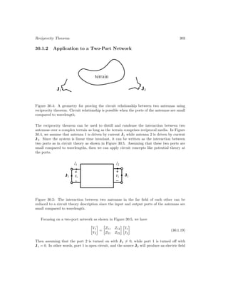
![304 Electromagnetic Field Theory
E2 at port 1. Consequently,
E2, J1 =
V
dV (E2 · J1) = I1
Port 1
E2 · dl = −I1V oc
1 (30.1.20)
Even though port 1 is assumed to be off, the J1 to be used above is the J1 when port 1
is turned on. Given that the port is in the circuit physics regime, then the current J1 is a
constant current at the port when it is turned on. The current J1 = ˆ
lI1/A where A is the
cross-sectional area of the wire, and ˆ
l is a unit vector aligned with the axis of the wire. The
volume integral dV = Adl, and hence the second equality follows above, where dl = ˆ
ldl. Since
Port 1
E2 · dl = −V oc
1 , we have the last equality above.
We can repeat the derivation with port 2 to arrive at
E1, J2 = I2
Port 2
E1 · dl = −I2V oc
2 (30.1.21)
But from (30.1.19), we can set the pertinent currents to zero to find these open circuit
voltages. Therefore, V oc
1 = Z12I2, V oc
2 = Z21I1. Since I1V oc
1 = I2V oc
2 by the reaction concept
or by reciprocity, then Z12 = Z21. The above analysis can be easily generalized to an N-port
network.
The simplicity of the above belies its importance. The above shows that the reciprocity
concept in circuit theory is a special case of reciprocity theorem for electromagnetic theory.
The terrain can also be replaced by complex circuits as in a circuit board, as long as the
materials are reciprocal, linear and time invariant. The complex terrain can also be replaced
by complex antenna structures.
30.1.3 Voltage Sources in Electromagnetics
Figure 30.6: Two ways to model voltage sources: (i) A current source Ja driving a very
short antenna, and (ii) A magnetic frill source (loop source) Ma driving a very short antenna
(courtesy of Kong, ELectromagnetic Wave Theory [31]).](https://image.slidesharecdn.com/emftall20191204-240115133321-d13ecad1/85/EMFTAll2-318-320.jpg)
![Reciprocity Theorem 305
In the above discussions, we have used current sources in reciprocity theorem to derive certain
circuit concepts. Before we end this section, it is prudent to mention how voltage sources are
modeled in electromagnetic theory. The use of the impressed currents so that circuit concepts
can be applied is shown in Figure 30.6. The antenna in (a) is driven by a current source.
But a magnetic current can be used as a voltage source in circuit theory as shown by Figure
30.6b. By using duality concept, an electric field has to curl around a magnetic current just
in Ampere’s law where magnetic field curls around an electric current. This electric field will
cause a voltage drop between the metal above and below the magnetic current loop making
it behave like a voltage source.5
30.1.4 Hind Sight
The proof of reciprocity theorem for Maxwell’s equations is very deeply related to the sym-
metry of the operator involved. We can see this from linear algebra. Given a matrix equation
driven by two different sources, they can be written succinctly as
A · x1 = b1 (30.1.22)
A · x2 = b2 (30.1.23)
We can left dot multiply the first equation with x2 and do the same with the second equation
with x1 to arrive at
xt
2 · A · x1 = xt
2 · b1 (30.1.24)
xt
1 · A · x2 = xt
1 · b2 (30.1.25)
If A is symmetric, the left-hand side of both equations are equal to each other. Subtracting
the two equations, we arrive at
xt
2 · b1 = xt
1 · b2 (30.1.26)
The above is analogous to the statement of the reciprocity theorem. The above inner product
is that of dot product in matrix theory, but the inner product for reciprocity is that for
infinite dimensional space. So if the operators in Maxwell’s equations are symmetrical, then
reciprocity theorem applies.
5More can be found in Jordain and Balmain, Electromagnetic Waves and Radiation Systems [48].](https://image.slidesharecdn.com/emftall20191204-240115133321-d13ecad1/85/EMFTAll2-319-320.jpg)
![306 Electromagnetic Field Theory
30.1.5 Transmit and Receive Patterns of an Antennna
Figure 30.7: The schematic diagram for studying the transmit and receive properties of
antennas.
Reciprocity also implies that the transmit and receive properties of an antenna is similar to
each other. Consider an antenna in the transmit mode. Then the radiation power density
that it will yield around the antenna is6
Srad =
Pt
4πr2
G(θ, φ) (30.1.27)
where Pt is the total power radiated by the transmit antenna, and G(θ, φ) is its directive gain
function. It is to be noted that in the above
4π
dΩG(θ, φ) = 4π.
Effective Gain versus Directive Gain
At this juncture, it is important to introduce the concept of effective gain versus directive
gain. The effective gain, also called the power gain, is
Ge(θ, φ) = feG(θ, φ) (30.1.28)
where fe is the efficiency of the antenna, a factor less than 1. It accounts for the fact that
not all power pumped into the antenna is delivered as radiated power. For instance, power
can be lost in the circuits and mismatch of the antenna. Therefore, the correct formula the
6The author is indebted to inspiration from E. Kudeki of UIUC for this part of the lecture notes [125].](https://image.slidesharecdn.com/emftall20191204-240115133321-d13ecad1/85/EMFTAll2-320-320.jpg)
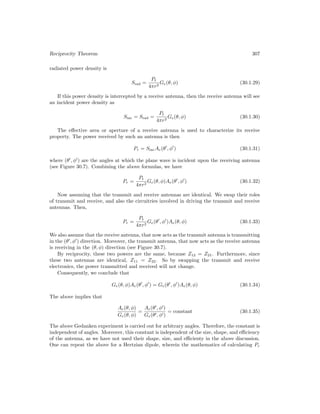
![308 Electromagnetic Field Theory
and Pt is a lot simpler. This constant is found to be λ2
/(4π).7
Therefore, an interesting
relationship between the effective aperture (or area) and the directive gain function is that
Ae(θ, φ) =
λ2
4π
Ge(θ, φ) (30.1.36)
One amusing point about the above formula is that the effective aperture, say of a Hertzian
dipole, becomes very large when the frequency is low, or the wavelength is very long. Of
course, this cannot be physically true, and I will let you meditate on this paradox and muse
over this point.
7See Kong [31][p. 700]. The derivation is for 100% efficient antenna. A thermal equilibrium argument is
used in [125] and Wikipedia [126] as well.](https://image.slidesharecdn.com/emftall20191204-240115133321-d13ecad1/85/EMFTAll2-322-320.jpg)
![Lecture 31
Equivalence Theorem, Huygens’
Principle
31.1 Equivalence Theorem or Equivalence Principle
Another theorem that is closely related to uniqueness theorem is the equivalence theorem or
equivalence principle. This theorem is discussed in many textbooks [31,47,48,59,154]. Some
authors also call it Love’s equivalence principle [155].
We can consider three cases: (1) The inside out case. (2) The outside in case. (3) The
general case.
31.1.1 Inside-Out Case
Figure 31.1: The inside-out problem where equivalent currents are impressed on the surface
S to produce the same fields outside in Vo in both cases.
In this case, we let J and M be the time-harmonic radiating sources inside a surface S
radiating into a region V = Vo ∪ Vi. They produce E and H everywhere. We can construct
309](https://image.slidesharecdn.com/emftall20191204-240115133321-d13ecad1/85/EMFTAll2-323-320.jpg)
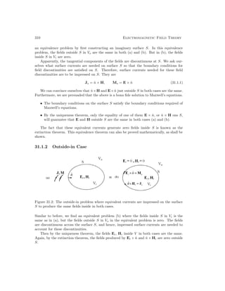
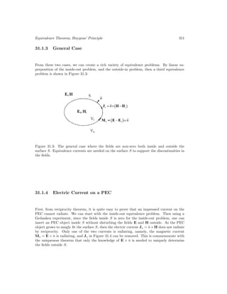
![312 Electromagnetic Field Theory
Figure 31.4: On a PEC surface, only one of the two currents is needed since an electric current
does not radiate on a PEC surface.
31.1.5 Magnetic Current on a PMC
Again, from reciprocity, an impressed magnetic current on a PMC cannot radiate. By the
same token, we can perform the Gedanken experiment as before by inserting a PMC object
inside S. It will not alter the fields outside S, as the fields inside S is zero. As the PMC
object grows to snugly fit the surface S, only the electric current Js = n̂ × H radiates, and
the magnetic current Ms = E × n̂ does not radiate and it can be removed. This is again
commensurate with the uniqueness theorem that only the knowledge of the n̂ × H is needed
to uniquely determine the fields outside S.
Figure 31.5: Similarly, on a PMC, only an electric current is needed to produce the field
outside the surface S.
31.2 Huygens’ Principle and Green’s Theorem
Huygens’ principle shows how a wave field on a surface S determines the wave field outside the
surface S. This concept was expressed by Huygens in the 1600s [156]. But the mathematical
expression of this idea was due to George Green1
in the 1800s. This concept can be expressed
1George Green (1793-1841) was self educated and the son of a miller in Nottingham, England [157].](https://image.slidesharecdn.com/emftall20191204-240115133321-d13ecad1/85/EMFTAll2-326-320.jpg)
![Equivalence Theorem, Huygens’ Principle 313
mathematically for both scalar and vector waves. The derivation for the vector wave case is
homomorphic to the scalar wave case. But the algebra in the scalar wave case is much simpler.
Therefore, we shall first discuss the scalar wave case first, followed by the electromagnetic
vector wave case.
31.2.1 Scalar Waves Case
Figure 31.6: The geometry for deriving Huygens’ principle for scalar wave equation.
For a ψ(r) that satisfies the scalar wave equation
(∇2
+ k2
) ψ(r) = 0, (31.2.1)
the corresponding scalar Green’s function g(r, r0
) satisfies
(∇2
+ k2
) g(r, r0
) = −δ(r − r0
). (31.2.2)
Next, we multiply (31.2.1) by g(r, r0
) and (31.2.2) by ψ(r). And then, we subtract the
resultant equations and integrating over a volume V as shown in Figure 31.6. There are two
cases to consider: when r0
is in V , or when r0
is outside V . Thus, we have
if r0
∈ V , ψ(r0
)
if r0
6∈ V , 0
=
V
dr [g(r, r0
)∇2
ψ(r) − ψ(r)∇2
g(r, r0
)], (31.2.3)
The left-hand side evaluates to different values depending on where r0
is due to the sifting
property of the delta function δ(r−r0
). Since g∇2
ψ−ψ∇2
g = ∇·(g∇ψ−ψ∇g), the left-hand](https://image.slidesharecdn.com/emftall20191204-240115133321-d13ecad1/85/EMFTAll2-327-320.jpg)
![314 Electromagnetic Field Theory
side of (31.2.3) can be rewritten using Gauss’ divergence theorem, giving2
if r
∈ V , ψ(r
)
if r
∈ V , 0
=
S
dS n̂ · [g(r, r
)∇ψ(r) − ψ(r)∇g(r, r
)], (31.2.4)
where S is the surface bounding V . The above is the mathematical expression that once ψ(r)
and n̂ · ∇ψ(r) are known on S, then ψ(r
) away from S could be found. This is similar to the
expression of equivalence principle where n̂ · ∇ψ(r) and ψ(r) are equivalence sources on the
surface S. In acoustics, these are known as single layer and double layer sources, respectively.
The above is also the mathematical expression of the extinction theorem that says if r
is
outside V , the left-hand side evaluates to zero.
In (31.2.4), the surface integral on the right-hand side can be thought of as contributions
from surface sources. Since g(r, r
) is a monopole Green’s function, the first term can be
thought of as radiation from single layer sources on the surface S. Also, since n̂ · ∇g(r, r
)
is the field due to a dipole, the second term is thought of as contributions from double layer
sources.
Figure 31.7: The geometry for deriving Huygens’ principle. The radiation from the source can
be replaced by equivalent sources on the surface S, and the field outside S can be calculated
using (31.2.4).
If the volume V is bounded by S and Sinf as shown in Figure 31.7, then the surface
integral in (31.2.4) should include an integral over Sinf . But when Sinf → ∞, all fields look
like plane wave, and ∇ → −r̂jk on Sinf . Furthermore, g(r − r
) ∼ O(1/r),3
when r → ∞,
2The equivalence of the volume integral in (31.2.3) to the surface integral in (31.2.4) is also known as
Green’s theorem [81].
3The symbol “O” means “of the order.”](https://image.slidesharecdn.com/emftall20191204-240115133321-d13ecad1/85/EMFTAll2-328-320.jpg)
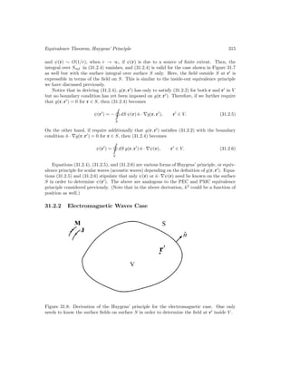
![316 Electromagnetic Field Theory
In a source-free region, an electromagnetic wave satisfies the vector wave equation
∇ × ∇ × E(r) − k2
E(r) = 0. (31.2.7)
The analogue of the scalar Green’s function for the scalar wave equation is the dyadic Green’s
function for the electromagnetic wave case [1, 31, 158, 159]. Moreover, the dyadic Green’s
function satisfies the equation4
∇ × ∇ × G(r, r0
) − k2
G(r, r0
) = I δ(r − r0
). (31.2.8)
It can be shown by direct back substitution that the dyadic Green’s function in free space
is [159]
G(r, r0
) =
I +
∇∇
k2
g(r − r0
) (31.2.9)
The above allows us to derive the vector Green’s theorem [1,31,158].
Then, after post-multiplying (31.2.7) by G(r, r0
), pre-multiplying (31.2.8) by E(r), sub-
tracting the resultant equations and integrating the difference over volume V , considering
two cases as we did for the scalar wave case, we have
if r0
∈ V , E(r0
)
if r0
6∈ V , 0
=
V
dV
E(r) · ∇ × ∇ × G(r, r0
)
−∇ × ∇ × E(r) · G(r, r0
)
. (31.2.10)
Next, using the vector identity that5
−∇ ·
E(r) × ∇ × G(r, r0
) + ∇ × E(r) × G(r, r0
)
= E(r) · ∇ × ∇ × G(r, r0
) − ∇ × ∇ × E(r) · G(r, r0
), (31.2.11)
Equation (31.2.10), with the help of Gauss’ divergence theorem, can be written as
if r0
∈ V , E(r0
)
if r0
6∈ V , 0
= −
S
dS n̂ ·
E(r) × ∇ × G(r, r0
) + ∇ × E(r) × G(r, r0
)
= −
S
dS
n̂ × E(r) · ∇ × G(r, r0
) + iωµ n̂ × H(r) · G(r, r0
)
. (31.2.12)
The above is just the vector analogue of (31.2.4). Since E × n̂ and n̂ × H are associated
with surface magnetic current and surface electric current, respectively, the above can be
4A dyad is an outer product between two vectors, and it behaves like a tensor, except that a tensor is more
general than a dyad. A purist will call the above a tensor Green’s function, as the above is not a dyad in its
strictest definition.
5This identity can be established by using the identity ∇ · (A × B) = B · ∇ × A − A · ∇ × B. We will have
to let (31.2.11) act on a constant vector to convert the dyad into a vector before we can apply this identity.
The equality of the volume integral in (31.2.10) to the surface integral in (31.2.12) is also known as vector
Green’s theorem [31,158]. Earlier form of this theorem was known as Franz formula [160].](https://image.slidesharecdn.com/emftall20191204-240115133321-d13ecad1/85/EMFTAll2-330-320.jpg)
![Equivalence Theorem, Huygens’ Principle 317
thought of having these equivalent surface currents radiating via the dyadic Green’s function.
Again, notice that (31.2.12) is derived via the use of (31.2.8), but no boundary condition has
yet been imposed on G(r, r0
) on S even though we have given a closed form solution for the
free-space case.
Now, if we require the addition boundary condition that n̂ × G(r, r0
) = 0 for r ∈ S. This
corresponds to a point source radiating in the presence of a PEC surface. Then (31.2.12)
becomes
E(r0
) = −
S
dS n̂ × E(r) · ∇ × G(r, r0
), r0
∈ V (31.2.13)
for it could be shown that n̂ × H · G = H · n̂ × G implying that the second term in (31.2.12)
is zero. On the other hand, if we require that n̂ × ∇ × G(r, r0
) = 0 for r ∈ S, then (31.2.12)
becomes
E(r0
) = −iωµ
S
dS n̂ × H(r) · G(r, r0
), r0
∈ V (31.2.14)
Equations (31.2.13) and (31.2.14) state that E(r0
) is determined if either n̂×E(r) or n̂×H(r) is
specified on S. This is in agreement with the uniqueness theorem. These are the mathematical
expressions of the PEC and PMC equivalence problems we have considered in the previous
sections.
The dyadic Green’s functions in (31.2.13) and (31.2.14) are for a closed cavity since bound-
ary conditions are imposed on S for them. But the dyadic Green’s function for an unbounded,
homogeneous medium, given in (31.2.10) can be written as
G(r, r0
) =
1
k2
[∇ × ∇ × I g(r − r0
) − I δ(r − r0
)], (31.2.15)
∇ × G(r, r0
) = ∇ × I g(r − r0
). (31.2.16)
Then, (31.2.12), for r0
∈ V and r0
6= r, becomes
E(r0
) = −∇0
×
S
dS g(r − r0
) n̂×E(r) +
1
iω
∇0
×∇0
×
S
dS g(r − r0
) n̂×H(r). (31.2.17)
The above can be applied to the geometry in Figure 31.7 where r0
is enclosed in S and Sinf .
However, the integral over Sinf vanishes by virtue of the radiation condition as for (31.2.4).
Then, (31.2.17) relates the field outside S at r0
in terms of only the field on S. This is similar
to the inside-out problem in the equivalence theorem. It is also related to the fact that if the
radiation condition is satisfied, then the field outside of the source region is uniquely satisfied.
Hence, this is also related to the uniqueness theorem.](https://image.slidesharecdn.com/emftall20191204-240115133321-d13ecad1/85/EMFTAll2-331-320.jpg)

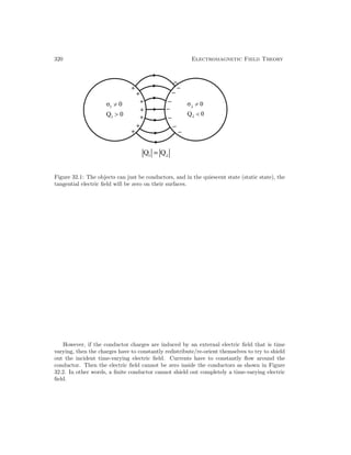
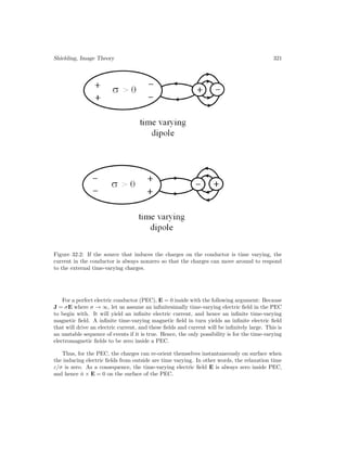
![322 Electromagnetic Field Theory
32.2 Image Theory
Image theory can be used to derived closed form solution to boundary value problems when
the geometry is simple and has a lot of symmetry. The closed form solutions in turn offer
physical insight into the problems. This theory or method is also discussed in many textbooks
[1,48,59,71,154,161,162].
32.2.1 Electric Charges and Electric Dipoles
Image theory for a flat conductor surface or a half-space is quite easy to derive. To see that,
we can start with electro-static theory of putting a positive charge above a flat plane. As
mentioned before, for electrostatics, the plane or half-space does not have to be a perfect
conductor, but only a conductor (or a metal). The tangential static electric field on the
surface of the conductor has to be zero.
The tangential static electric field can be canceled by putting an image charge of opposite
sign at the mirror location of the original charge. This is shown in Figure 32.3. Now we can
mentally add the total field due to these two charges. When the total static electric field due
to the original charge and image charge is sketched, it will look like that in Figure 32.4. It
is seen that the static electric field satisfies the boundary condition that n̂ × E = 0 at the
conductor interface due to symmetry.](https://image.slidesharecdn.com/emftall20191204-240115133321-d13ecad1/85/EMFTAll2-336-320.jpg)
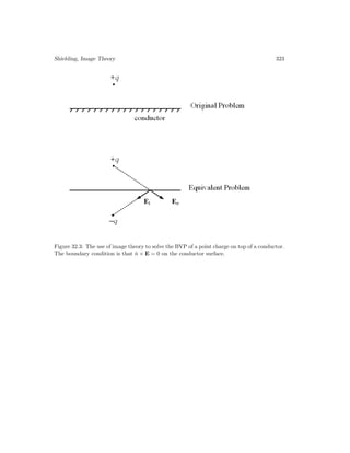
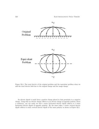

![326 Electromagnetic Field Theory
Figure 32.6: On a PEC surface, n̂ · B = 0. Hence, a magnetic monopole on top of a PEC
surface will have magnetic field distributed as shown.
By extrapolating this to magnetic dipoles, they will reflect themselves to the magnetic
dipoles as shown in Figure 32.7. A horizontal magnetic dipole reflects to a horizontal magnetic
dipole of the same polarity, and a vertical magnetic dipole reflects to a vertical magnetic dipole
of opposite polarity. Hence, a dipolar bar magnet can be levitated by a superconductor when
this magnet is placed closed to it. This is also known as the Meissner effect [163], which is
shown in Figure 32.8.
A time-varying magnetic dipole can be made from a electric current loop. Over a PEC, a
time-varying magnetic dipole will reflect the same way as a static magnetic dipole as shown
in Figure 32.7.](https://image.slidesharecdn.com/emftall20191204-240115133321-d13ecad1/85/EMFTAll2-340-320.jpg)
![Shielding, Image Theory 327
Figure 32.7: Using the rule of how magnetic monopole reflects itself on a PEC surface, the
reflection rules for magnetic dipoles can be ascertained.
Figure 32.8: On a PEC (superconducting) surface, a vertical magnetic dipole reflects to one
of opposite polarity. Hence, the dipoles repel each other displaying the Meissner effect. The
magnet, because of the repulsive force from its image, levitates above the superconductor
(courtesy of Wikipedia [164]).
32.2.3 Perfect Magnetic Conductor (PMC) Surfaces
Magnetic conductor does not come naturally in this world since there are no free-moving
magnetic charges around. Magnetic monopoles are yet to be discovered. On a PMC surface,](https://image.slidesharecdn.com/emftall20191204-240115133321-d13ecad1/85/EMFTAll2-341-320.jpg)
![328 Electromagnetic Field Theory
by duality, n̂ × H = 0. At low frequency, it can be mimicked by a high µ material. One can
see that for magnetostatics, at the interface of a high µ material and air, the magnetic flux is
approximately normal to the surface, resembling a PMC surface. High µ materials are hard
to find at higher frequencies. Since n̂ × H = 0 on such a surface, no electric current can flow
on such a surface. Hence, a PMC can be mimicked by a surface where no surface electric
current can flow. This has been achieved in microwave engineering with a mushroom surface
as shown in Figure 32.9 [165]. The mushroom structure consisting of a wire and an end-cap,
can be thought of as forming an LC tank circuit. Close to the resonance frequency of this
tank circuit, the surface of mushroom structures essentially becomes open circuits resembling
a PMC. Therefore, there is no surface electric current on this surface, and the tangential
magnetic field is small, the hallmark of a good magnetic conductor.
Figure 32.9: A mushroom structure operates like an LC tank circuit. At the right frequency,
the surface resembles an open-circuit surface where no current can flow. Hence, tangential
magnetic field is zero resembling perfect magnetic conductor (courtesy of Sievenpiper [165]).
Mathematically, a surface that is dual to the PEC surface is the perfect magnetic conductor
(PMC) surface. The magnetic dipole is also dual to the electric dipole. Thus, over a PMC
surface, these electric and magnetic dipoles will reflect differently as shown in Figure 32.10.
One can go through Gedanken experiments and verify that the reflection rules are as shown
in the figure.](https://image.slidesharecdn.com/emftall20191204-240115133321-d13ecad1/85/EMFTAll2-342-320.jpg)
![Shielding, Image Theory 329
Figure 32.10: Reflection rules for electric and magnetic dipoles over a PMC surface.
Figure 32.11: Image theory for multiple images [29].
32.2.4 Multiple Images
For the geometry shown in Figure 32.11, one can start with electrostatic theory, and convince
oneself that n̂ × E = 0 on the metal surface with the placement of charges as shown. For
conducting media, they charges will relax to the quiescent distribution after the relaxation
time. For PEC surfaces, one can extend these cases to time-varying dipoles because the
charges in the PEC medium can re-orient instantaneously (i.e. with zero relaxation time) to
shield out or expel the E and H fields. Again, one can repeat the above exercise for magnetic
charges, magnetic dipoles, and PMC surfaces.](https://image.slidesharecdn.com/emftall20191204-240115133321-d13ecad1/85/EMFTAll2-343-320.jpg)
![330 Electromagnetic Field Theory
Figure 32.12: Image theory for a point charge near a cylinder or a sphere can be found in
closed form [29].
32.2.5 Some Special Cases
One curious case is for a static charge placed near a conductive sphere (or cylinder) as shown in
Figure 32.12.2
A charge of +Q reflects to a charge of −QI inside the sphere. For electrostatics,
the sphere (or cylinder) need only be a conductor. However, this cannot be generalized to
electrodynamics or a time-varying problem, because of the retardation effect: A time-varying
dipole or charge will be felt at different points asymmetrically on the surface of the sphere
from the original and image charges. Exact cancelation of the tangential electric field cannot
occur for time-varying field.
Figure 32.13: A static charge over a dielectric interface can be found in closed form.
When a static charge is placed over a dielectric interface, image theory can be used to
find the closed form solution. This solution can be derived using Fourier transform technique
which we shall learn later [34]. It can also be extended to multiple interfaces. But image
theory cannot be used for the electrodynamic case due to the different speed of light in
different media, giving rise to different retardation effects.
2This is worked out in p. 48 and p. 49, Ramo et al [29].](https://image.slidesharecdn.com/emftall20191204-240115133321-d13ecad1/85/EMFTAll2-344-320.jpg)
![Lecture 33
High Frequency Solutions,
Gaussian Beams
33.1 High Frequency Solutions
High frequency solutions are important in many real-world applications. This occurs when the
wavelength is much smaller than the size of the structure. This can occur even in microwave
interacting with reflector antennas for instance. It is also the transition from waves regime
to the optics regime in the solutions of Maxwell’s equations. Often times, the term “quasi-
optical” is used to describe the solutions in this regime.
33.1.1 Tangent Plane Approximations
We have learnt that reflection and transmission of waves at a flat surface can be solved in
closed form. The important point here is the physics of phase matching. Due to phase
matching, we have the law of reflection, transmission and Snell’s law [52].1
When a surface is not flat anymore, there is no closed form solution. But when a surface is
curved, an approximate solution can be found. This is obtained by using a local tangent-plane
approximation when the radius of curvature is much larger than the wavelength. Hence, this
is a good approximation when the frequency is high or the wavelength is short. This is similar
in spirit that we can approximate a spherical wave by a local plane wave at the spherical wave
front when the wavelength is short.
When the wavelength is short, phase matching happens locally, and the law of reflection,
transmission, and Snell’s law are satisfied approximately as shown in Figure 33.1. The tangent
plane approximation is the basis for the geometrical optics (GO) approximation [31,167]. In
GO, light waves are replaced by light rays. The reflection and transmission of these rays at
an interface is estimated with the tangent plane approximation. This is also the basis for lens
or ray optics from which lens technology is derived. It is also the basis for ray tracing for
high-frequency solutions [168,169].
1This law is also known in the Islamic world in 984 [166].
331](https://image.slidesharecdn.com/emftall20191204-240115133321-d13ecad1/85/EMFTAll2-345-320.jpg)
![332 Electromagnetic Field Theory
Most of these problems do not have closed-form solutions, and have to be treated with ap-
proximate methods. In addition to geometrical approximations mentioned above, asymptotic
methods are also used to find approximate solutions. Asymptotic methods implies finding
a solution when there is a large parameter in the problem. In this case, it is usually the
frequency. Such high-frequency approximate methods are discussed in [170–174].
Figure 33.1: In the tangent plane approximation, the surface where reflection and refraction
occur is assumed to be locally flat. Hence, phase-matching is approximately satisfied, and
hence, the law of reflection, transmittion, and Snell’s law.
33.1.2 Fermat’s Principle
Fermat’s principle (1600s) [52,175] says that a light ray follows the path that takes the shortest
time between two points.2
Since time delay is related to the phase delay, and that a light ray
can be locally approximated by a plane wave, this can be stated that a plane wave follows the
path that has a minimal phase delay. This principle can be used to derive law of reflection,
transmission, and refraction for light rays. It can be used as the guiding principle for ray
tracing.
2This eventually give rise to the principle of least action.](https://image.slidesharecdn.com/emftall20191204-240115133321-d13ecad1/85/EMFTAll2-346-320.jpg)
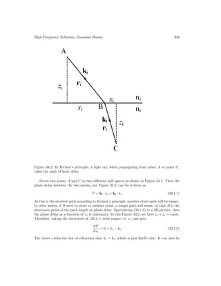
![334 Electromagnetic Field Theory
obtained by phase matching. Notice that in the above, only xi is varied to find the stationary
point and ki and kt remain constant.
33.1.3 Generalized Snell’s Law
Figure 33.3: A phase screen which is position dependent can be made. In such a case, one
can derive a generalized Snell’s law to describe the diffraction of a wave by such a surface
(courtesy of Capasso’s group [176]).
Metasurfaces are prevalent these days due to our ability for nano-fabrication and numerical
simulation. One of them is shown in Figure 33.3. Such a metasurface can be thought of as a
phase screen, providing additional phase shift for the light as it passes through it. Moreover,
the added phase shift can be controlled to be a function of position due to advent in fabrication
technology and commercial software for numerical simulation.
To model this phase screen, we can add an additional function Φ(x, y) to (33.1.1), namely
that
P = ki · ri + kt · rt − Φ(xi, yi) (33.1.3)
Now applying Fermat’s principle that there should be minimal phase delay, and taking the
derivative of the above with respect to xi, one gets
∂P
∂xi
= ki − kt −
∂Φ(xi, yi)
∂xi
= 0 (33.1.4)
The above yields that the generalized Snell’s law [176] that
ki − kt =
∂Φ(xi, yi)
∂xi
(33.1.5)
It yields the fact that the transmitted light can be directed to other angles due to the
additional phase screen.](https://image.slidesharecdn.com/emftall20191204-240115133321-d13ecad1/85/EMFTAll2-348-320.jpg)
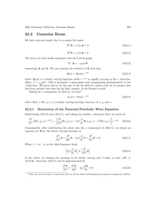
![336 Electromagnetic Field Theory
The above is called the paraxial wave equation. It is also called the parabolic wave equation.4
It implies that the β vector of the wave is approximately parallel to the z axis, and hence,
the name.
33.2.2 Finding a Closed Form Solution
A closed form solution to the paraxial wave equation can be obtained by a simple trick5
. It
is known that
Ax(r) =
e−jβ|r−r0
|
4π|r − r0|
(33.2.10)
is the solution to
∇2
Ax + β2
Ax = 0 (33.2.11)
if r 6= r0
. If we make r0
= −ẑjb, a complex number, then (33.2.10) is always a solution to
(33.2.10) for all r, because |r − r0
| 6= 0 always. Then
|r − r0
| =
p
x2 + y2 + (z + jb)2
≈ (z + jb)
1 +
x2
+ y2
(z + jb)2
+ . . .
1/2
≈ (z + jb) +
x2
+ y2
2(z + jb)
+ . . . , |z + jb| → ∞ (33.2.12)
And then
Ax(r) ≈
e−jβ(z+jb)
4π(z + jb)
e−jβ x2+y2
2(z+jb) (33.2.13)
By comparing the above with (33.2.5), we can identify
Ψ(x, y, z) = A0
jb
z + jb
e−jβ x2+y2
2(z+jb) (33.2.14)
By separating the exponential part into the real part and the imaginary part, and writing
the prefactor in terms of amplitude and phase, we have
Ψ(x, y, z) =
A0
p
1 + z2/b2
ej tan−1
( z
b )
e
−jβ x2+y2
2(z2+b2)
z
e
−bβ x2+y2
2(z2+b2) (33.2.15)
The above can be rewritten as
Ψ(x, y, z) =
A0
p
1 + z2/b2
e−jβ x2+y2
2R e− x2+y2
w2
ejψ
(33.2.16)
4The paraxial wave equation, the diffusion equation and the Schrodinger equation are all classified as
parabolic equations in mathematical parlance [34,43,177,178].
5Introduced by Georges A. Deschamps of UIUC [179].](https://image.slidesharecdn.com/emftall20191204-240115133321-d13ecad1/85/EMFTAll2-350-320.jpg)
![High Frequency Solutions, Gaussian Beams 337
where A0 is a new constant introduced to absorb undesirable constants arising out of the
algebra, and
w2
=
2b
β
1 +
z2
b2
, R =
z2
+ b2
z
, ψ = tan−1
z
b
(33.2.17)
For a fixed z, the parameters w, R, and ψ are constants. Here, w is the beam waist which
varies with z, and it is smallest when z = 0, or w = w0 =
2b
β . And R is the radius of
curvature of the constant phase front. This can be appreciated by studying a spherical wave
front e−jβR
, and make a paraxial wave approximation, namely, x2
+ y2
z2
to get
e−jβR
= e−jβ(x2
+y2
+z2
)1/2
= e
−jβz
1+ x2+y2
z2
1/2
≈ e−jβz−jβ x2+y2
2z ≈ e−jβz−jβ x2+y2
2R (33.2.18)
In the last approximation, we assume that z ≈ R in the paraxial approximation. The phase
ψ changes rapidly with z.
A cross section of the electric field due to a Gaussian beam is shown in Figure 33.4.
Figure 33.4: Electric field of a Gaussian beam in the x − z plane frozen in time. The wave
moves to the right as time increases; b/λ = 10/6 (courtesy of Haus, Electromagnetic Noise
and Quantum Optical Measurements [74]).
33.2.3 Other solutions
In general, the paraxial wave equation has solution of the form6
Ψnm(x, y, z) =
2
πn!m!
1/2
2−N/2
1
w
e−(x2
+y2
)/w2
e−j β
2R (x2
+y2
)
ej(m+n+1)Ψ
·Hn
x
√
2/w
Hm
y
√
2/w
(33.2.19)
6See F. Pampaloni and J. Enderlein [180].](https://image.slidesharecdn.com/emftall20191204-240115133321-d13ecad1/85/EMFTAll2-351-320.jpg)
![338 Electromagnetic Field Theory
where Hn(ξ) is a Hermite polynomial of order n. The solution can also be express in terms
of Laguere polynomials, namely,
Ψnm(x, y, z) =
2
πn!m!
1/2
min(n, m)!
1
w
e−j β
2R ρ2
− e−ρ2
/w2
e+j(n+m+1)Ψ
ejlφ
(−1)min(n,m)
√
2ρ
w
Ln−m
min(n,m)
2ρ2
w2
(33.2.20)
where Lk
n(ξ) is the associated Laguerre polynomial.
These gaussian beams have rekindled recent excitement in the community because, in
addition to carrying spin angular momentum as in a plane wave, they can carry orbital
angular momentum due to the complex transverse field distribution of the beams.7
They
harbor potential for optical communications as well as optical tweezers to manipulate trapped
nano-particles. Figure 33.5 shows some examples of the cross section (xy plane) field plots
for some of these beams.
Figure 33.5: Examples of structured light. It can be used in encoding more information in
optical communications (courtesy of L. Allen and M. Padgett’s chapter in J.L. Andrew’s book
on structured light [181].
7See D.L. Andrew, Structured Light and Its Applications and articles therein [181].](https://image.slidesharecdn.com/emftall20191204-240115133321-d13ecad1/85/EMFTAll2-352-320.jpg)
![340 Electromagnetic Field Theory
Figure 34.1: The magnificent beauty of nature can be partly explained by Rayleigh scattering
[182,183].
When a ray of light impinges on an object, we model the incident light as a plane elec-
tromagnetic wave (see Figure 34.2). Without loss of generality, we can assume that the
electromagnetic wave is polarized in the z direction and propagating in the x direction. We
assume the particle to be a small spherical particle with permittivity εs and radius a. Essen-
tially, the particle sees a constant field as the plane wave impinges on it. In other words, the
particle feels an almost electrostatic field in the incident field.
Figure 34.2: Geometry for studying the Rayleigh scattering problem.](https://image.slidesharecdn.com/emftall20191204-240115133321-d13ecad1/85/EMFTAll2-354-320.jpg)
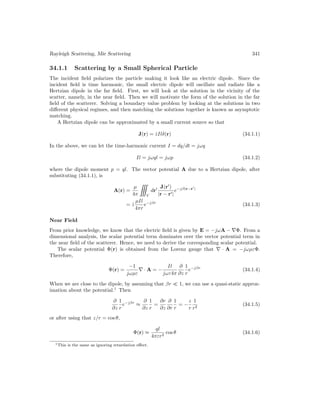
![342 Electromagnetic Field Theory
This dipole induced in the small particle is formed in response to the incident field. The
incident field can be approximated by a constant local static electric field,
Einc = ẑEi (34.1.7)
The corresponding electrostatic potential for the incident field is then2
Φinc = −zEi (34.1.8)
so that Einc ≈ −∇Φinc = ẑEi, as ω → 0. The scattered dipole potential from the spherical
particle in the vicinity of it is given by
Φsca = Es
a3
r2
cos θ (34.1.9)
The electrostatic boundary value problem (BVP) has been previously solved and3
Es =
εs − ε
εs + 2ε
Ei (34.1.10)
Using (34.1.10) in (34.1.9), and comparing with(34.1.6), one can see that the dipole moment
induced by the incident field is that
p = ql = 4πε
εs − ε
εs + 2ε
a3
Ei (34.1.11)
Far Field
In the far field of the Hertzian dipole, we can start with
E = −jωA − ∇Φ = −jωA −
1
jωµε
∇∇ · A (34.1.12)
But when we are in the far field, A behaves like a spherical wave which in turn behaves
like a local plane wave if one goes far enough. Therefore, ∇ → −jβ = −jβr̂. Using this
approximation in (34.1.12), we arrive at
E = −jω
A −
ββ
β2
· A
= −jω(A − r̂r̂ · A) = −jω(θ̂Aθ + φ̂Aφ) (34.1.13)
where we have used r̂ = β/β.
34.1.2 Scattering Cross Section
From (34.1.3), we see that Aφ = 0 while
Aθ = −
jωµql
4πr
e−jβr
sin θ (34.1.14)
2It is not easier to get here from electrodynamics. One needs vector spherical harmonics [184].
3It was one of the homework problems.](https://image.slidesharecdn.com/emftall20191204-240115133321-d13ecad1/85/EMFTAll2-356-320.jpg)
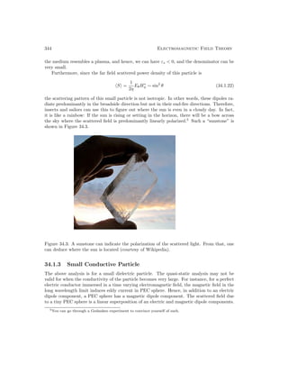
![Rayleigh Scattering, Mie Scattering 345
These two dipolar components have electric fields that cancel precisely at certain observation
angle. This gives rise to deep null in the bi-static radar scattering cross-section (RCS)6
of a
PEC sphere as illustrated in Figure 34.4.
Figure 34.4: RCS (radar scattering cross section) of a small PEC scatterer (courtesy of Sheng
et al. [185]).
34.2 Mie Scattering
When the size of the dipole becomes larger, quasi-static approximation is insufficient to
approximate the solution. Then one has to solve the boundary value problem in its full glory
usually called the full-wave theory or Mie theory [186,187]. With this theory, the scattering
cross section does not grow indefinitely with frequency. For a sphere of radius a, the scattering
cross section becomes πa2
in the high-frequency limit. This physical feature of this plot is
shown in Figure 34.5, and it also explains why the sky is not purple.
6Scattering cross section in microwave range is called an RCS due to its prevalent use in radar technology.](https://image.slidesharecdn.com/emftall20191204-240115133321-d13ecad1/85/EMFTAll2-359-320.jpg)
![346 Electromagnetic Field Theory
Figure 34.5: Radar cross section (RCS) calculated using Mie scattering theory [187].
34.2.1 Optical Theorem
Before we discuss Mie scattering solutions, let us discuss an amazing theorem called the
optical theorem. This theorem says that the scattering cross section of a scatterer depends
only on the forward scattering power density of the scatterer. In other words, if a plane wave
is incident on a scatterer, the scatterer will scatter the incident power in all directions. But
the total power scattered by the object is only dependent on the forward scattering power
density of the object or scatterer. This amazing theorem is called the optical theorem, and
the proof of this is given in J.D. Jackson’s book [42].
The true physical reason for this is power orthogonality. Two plane waves can interact or
exchange power with each other unless they share the same k or β vector. This happens in
orthogonal modes in waveguides [75,188].
The scattering pattern of a scatterer for increasing frequency is shown in Figure 34.6. For
Rayleigh scattering where the wavelength is long, the scattered power is distributed isotrop-
ically save for the doughnut shape of the radiation pattern, namely, the sin2
(θ) dependence.
As the frequency increases, the power is scattered increasingly in the forward direction. The
reason being that for very short wavelength, the scatterer looks like a disc to the incident
wave, casting a shadow in the forward direction. Hence, there has to be scattered field in the
forward direction to cancel the incident wave to cast this shadow.](https://image.slidesharecdn.com/emftall20191204-240115133321-d13ecad1/85/EMFTAll2-360-320.jpg)
![Rayleigh Scattering, Mie Scattering 347
In a nutshell, the scattering theorem is intuitively obvious for high-frequency scattering.
The amazing part about this theorem is that it is true for all frequencies.
Figure 34.6: A particle scatters increasingly more in the forward direction as the frequency
increases.Courtesy of hyperphysics.phy-astr.gsu.edu.
34.2.2 Mie Scattering by Spherical Harmonic Expansions
As mentioned before, as the wavelength becomes shorter, we need to solve the boundary
value problem in its full glory without making any approximations. This can be done by
using separation of variables and spherical harmonic expansions that will be discussed in the
section.
The Mie scattering solution by a sphere is beyond the scope of this course.7
This problem
have to solved by the separation of variables in spherical coordinates. The separation of
variables in spherical coordinates is not the only useful for Mie scattering, it is also useful for
analyzing spherical cavity. So we will present the precursor knowledge so that you can read
further into Mie scattering theory if you need to in the future.
34.2.3 Separation of Variables in Spherical Coordinates
To this end, we look at the scalar wave equation (∇2
+β2
)Ψ(r) = 0 in spherical coordinates. A
lookup table can be used to evaluate ∇·∇, or divergence of a gradient in spherical coordinates.
Hence, the Helmholtz wave equation becomes8
1
r2
∂
∂r
r2 ∂
∂r
+
1
r2 sin θ
∂
∂θ
sin θ
∂
∂θ
+
1
r2 sin2
θ
∂2
∂φ2
+ β2
Ψ(r) = 0 (34.2.1)
Noting the ∂2
/∂φ2
derivative, by using separation of variables technique, we assume Ψ(r) to
be
Ψ(r) = F(r, θ)ejmφ
(34.2.2)
7But it is treated in J.A. Kong’s book [31] and Chapter 3 of W.C. Chew, Waves and Fields in Inhomogeneous
Media [34] and many other textbooks [42,59,154].
8By quirk of mathematics, it turns out that the first term on the right-hand side below can be simplified
by observing that 1
r2
∂
∂r
r2 = 1
r
∂
∂r
r.](https://image.slidesharecdn.com/emftall20191204-240115133321-d13ecad1/85/EMFTAll2-361-320.jpg)
![348 Electromagnetic Field Theory
where ∂2
∂φ2 ejmφ
= −m2
ejmφ
. Then (34.2.1) becomes
1
r2
∂
∂r
r2 ∂
∂r
+
1
r2 sin θ
∂
∂θ
sin θ
∂
∂θ
−
m2
r2 sin2
θ
+ β2
F(r, θ) = 0 (34.2.3)
Again, by using the separation of variables, and letting further that
F(r, θ) = bn(βr)Pm
n (cos θ) (34.2.4)
where we require that
1
sin θ
d
dθ
sin θ
d
dθ
+
n(n + 1) −
m2
sin2
θ
Pm
n (cos θ) = 0 (34.2.5)
when Pm
n (cos θ) is the associate Legendre polynomial. Note that (34.2.5) is an eigenvalue
problem, and |m| ≤ |n|.
Consequently, bn(kr) satisfies
1
r2
d
dr
r2 d
dr
−
n(n + 1)
r2
+ β2
bn(βr) = 0 (34.2.6)
The above is the spherical Bessel equation where bn(βr) is either the spherical Bessel function
jn(βr), spherical Neumann function nn(βr), or the spherical Hankel functions, h
(1)
n (βr) and
h
(2)
n (βr). The spherical functions are related to the cylindrical functions via [34,43] 9
bn(βr) =
r
π
2βr
Bn+ 1
2
(βr) (34.2.7)
It is customary to define the spherical harmonic as
Ynm(θ, φ) =
s
2n + 1
4π
(n − m)!
(n + m)!
Pm
n (cos θ)ejmφ
(34.2.8)
The above is normalized such that
Yn,−m(θ, φ) = (−1)m
Y ∗
nm(θ, φ) (34.2.9)
and that
2π
0
dφ
π
0
sin θdθY ∗
n0m0 (θ, φ)Ynm(θ, φ) = δn0nδm0m (34.2.10)
These functions are also complete10
if like Fourier series, so that
∞
X
n=0
n
X
m=−n
Y ∗
nm(θ0
, φ0
)Ynm(θ, φ) = δ(φ − φ
0
)δ(cos θ − cos θ
0
) (34.2.11)
9By a quirk of nature, the spherical Bessel functions needed for 3D wave equations are in fact simpler than
cylindrical Bessel functions needed for 2D wave equation. One can say that 3D is real, but 2D is surreal.
10In a nutshell, a set of basis functions is complete in a subspace if any function in the same subspace can
be expanded as a sum of these basis functions.](https://image.slidesharecdn.com/emftall20191204-240115133321-d13ecad1/85/EMFTAll2-362-320.jpg)
![Lecture 35
Sommerfeld Integral, Weyl
Identity
35.1 Spectral Representations of Sources
A plane wave is a mathematical idealization that does not exist in the real world. In practice,
waves are nonplanar in nature as they are generated by finite sources, such as antennas
and scatterers. For example, a point source generates a spherical wave which is nonplanar.
Fortunately, these waves can be expanded in terms of sum of plane waves. Once this is done,
then the study of non-plane-wave reflections from a layered medium becomes routine. In the
following, we shall show how waves resulting from a point source can be expanded in terms of
plane waves summation. This topic is found in many textbooks [1,31,34,87,88,154,177,189].
35.1.1 A Point Source
From this point onward, we will adopt the exp(−iωt) time convention to be commensurate
with the optics and physics literatures.
There are a number of ways to derive the plane wave expansion of a point source. We will
illustrate one of the ways. The spectral decomposition or the plane-wave expansion of the
field due to a point source could be derived using Fourier transform technique. First, notice
that the scalar wave equation with a point source is
∂2
∂x2
+
∂2
∂y2
+
∂2
∂z2
+ k2
0
φ(x, y, z) = −δ(x) δ(y) δ(z). (35.1.1)
The above equation could then be solved in the spherical coordinates, yielding the solution
φ(r) =
eik0r
4πr
. (35.1.2)
349](https://image.slidesharecdn.com/emftall20191204-240115133321-d13ecad1/85/EMFTAll2-363-320.jpg)
![350 Electromagnetic Field Theory
Next, assuming that the Fourier transform of φ(x, y, z) exists, we can write
φ(x, y, z) =
1
(2π)3
∞
−∞
dkxdkydkz φ̃(kx, ky, kz)eikxx+ikyy+ikzz
. (35.1.3)
Then we substitute the above into (35.1.1), after exchanging the order of differentiation and
integration, one can convert
∂2
∂x2
+
∂2
∂y2
+
∂2
∂z2
= −k2
x − k2
y − k2
z
Then, together with the Fourier representation of the delta function, which is
δ(x) δ(y) δ(z) =
1
(2π)3
∞
−∞
dkxdkydkz eikxx+ikyy+ikzz
(35.1.4)
we convert (35.1.1) into
∞
−∞
dkxdkydkz [k2
0 − k2
x − k2
y − k2
z]φ̃(kx, ky, kz)eikxx+ikyy+ikzz
(35.1.5)
= −
∞
−∞
dkxdkydkz eikxx+ikyy+ikzz
. (35.1.6)
Since the above is equal for all x, y, and z, we can Fourier inverse transform the above to get
φ̃(kx, ky, kz) =
−1
k2
0 − k2
x − k2
y − k2
z
. (35.1.7)
Consequently, we have
φ(x, y, z) =
−1
(2π)3
∞
−∞
dk
eikxx+ikyy+ikzz
k2
0 − k2
x − k2
y − k2
z
. (35.1.8)](https://image.slidesharecdn.com/emftall20191204-240115133321-d13ecad1/85/EMFTAll2-364-320.jpg)
![Sommerfeld Integral, Weyl Identity 351
C
Re [kz]
– k2
0 – k2
x – k2
y
⊗
Fourier Inversion Contour
Im [kz]
k2
0 – k2
x – k2
y
×
Figure 35.1: The integration along the real axis is equal to the integration along C plus the
residue of the pole at (k2
0 − k2
x − k2
y)1/2
, by invoking Jordan’s lemma.
In the above, if we examine the kz integral first, then the integrand has poles at kz =
±(k2
0 − k2
x − k2
y)1/2
.1
Moreover, for real k0, and real values of kx and ky, these two poles
lie on the real axis, rendering the integral in (35.1.8) undefined. However, if a small loss is
assumed in k0 such that k0 = k
0 + ik
0 , then the poles are off the real axis (see Figure 35.1),
and the integrals in (35.1.8) are well-defined. As we shall see, this is intimately related to
the uniqueness principle we have studied before. First, the reason is that φ(x, y, z) is not
strictly absolutely integrable for a lossless medium, and hence, its Fourier transform may not
exist [45]. Second, the introduction of a small loss also guarantees the radiation condition
and the uniqueness of the solution to (35.1.1), and therefore, the equality of (35.1.2) and
(35.1.8) [34].
Observe that in (35.1.8), when z 0, the integrand is exponentially small when m[kz] →
∞. Therefore, by Jordan’s lemma, the integration for kz over the contour C as shown in Figure
35.1 vanishes. Then, by Cauchy’s theorem, the integration over the Fourier inversion contour
on the real axis is the same as integrating over the pole singularity located at (k2
0 −k2
x −k2
y)1/2
,
yielding the residue of the pole (see Figure 35.1). Consequently, after doing the residue
evaluation, we have
φ(x, y, z) =
i
2(2π)2
∞
−∞
dkxdky
eikxx+ikyy+ik
zz
k
z
, z 0, (35.1.9)
where k
z = (k2
0 − k2
x − k2
y)1/2
.
1In (35.1.8), the pole is located at k2
x + k2
y + k2
z = k2
0. This equation describes a sphere in k space, known
as the Ewald’s sphere [190].](https://image.slidesharecdn.com/emftall20191204-240115133321-d13ecad1/85/EMFTAll2-365-320.jpg)
![352 Electromagnetic Field Theory
Similarly, for z 0, we can add a contour C in the lower-half plane that contributes to
zero to the integral, one can deform the contour to pick up the pole contribution. Hence, the
integral is equal to the pole contribution at k0
z = −(k2
0 − k2
x − k2
y)1/2
(see Figure 35.1). As
such, the result for all z can be written as
φ(x, y, z) =
i
2(2π)2
∞
−∞
dkxdky
eikxx+ikyy+ik0
z|z|
k0
z
, all z. (35.1.10)
By the uniqueness of the solution to the partial differential equation (35.1.1) satisfying
radiation condition at infinity, we can equate (35.1.2) and (35.1.10), yielding the identity
eik0r
r
=
i
2π
∞
−∞
dkxdky
eikxx+ikyy+ikz|z|
kz
, (35.1.11)
where k2
x +k2
y +k2
z = k2
0, or kz = (k2
0 −k2
x −k2
y)1/2
. The above is known as the Weyl identity
(Weyl 1919). To ensure the radiation condition, we require that =m[kz] 0 and e[kz] 0
over all values of kx and ky in the integration. Furthermore, Equation (35.1.11) could be
interpreted as an integral summation of plane waves propagating in all directions, including
evanescent waves. It is the plane-wave expansion of a spherical wave.
Figure 35.2: The wave is propagating for kρ vectors inside the disk, while the wave is evanes-
cent for kρ outside the disk.
One can also interpret the above as a 2D surface integral in the Fourier space over the kx
and ky variables. When k2
x +k2
y k2
0, or inside a disk of radius k0, the waves are propagating](https://image.slidesharecdn.com/emftall20191204-240115133321-d13ecad1/85/EMFTAll2-366-320.jpg)
![Sommerfeld Integral, Weyl Identity 353
waves. But for contributions outside this disk, the waves are evanescent (see Figure 35.2).
And the high Fourier (or spectral) components of the Fourier spectrum correspond to evanes-
cent waves. Since high spectral components, which are related to the evanescent waves, are
important for reconstructing the singularity of the Green’s function.
y
kρ
a
φ x
ρ
Figure 35.3: The kρ and the ρ vector on the xy plane.
In (35.1.11), we can write kρ = x̂kρ cos α + ŷkρ sin α, ρ = x̂ρ cos φ + ŷρ sin φ (see Figure
35.3), and dkxdky = kρdkρ dα. Then, kxx + kyy = kρ · ρ = kρ cos(α − φ), and we have
eik0r
r
=
i
2π
∞
0
kρdkρ
2π
0
dα
eikρρ cos(α−φ)+ikz|z|
kz
, (35.1.12)
where kz = (k2
0 −k2
x −k2
y)1/2
= (k2
0 −k2
ρ)1/2
, where in cylindrical coordinates, in the kρ-space,
or the Fourier space, k2
ρ = k2
x + k2
y. Then, using the integral identity for Bessel functions
given by2
J0(kρρ) =
1
2π
2π
0
dα eikρρ cos(α−φ)
, (35.1.13)
(35.1.12) becomes
eik0r
r
= i
∞
0
dkρ
kρ
kz
J0(kρρ)eikz|z|
. (35.1.14)
The above is also known as the Sommerfeld identity (Sommerfeld 1909 [192]; [177][p. 242]).
Its physical interpretation is that a spherical wave can be expanded as an integral summation
of conical waves or cylindrical waves in the ρ direction, times a plane wave in the z direction
over all wave numbers kρ. This wave is evanescent in the ±z direction when kρ k0.
2See Chew [34], or Whitaker and Watson(1927) [191].](https://image.slidesharecdn.com/emftall20191204-240115133321-d13ecad1/85/EMFTAll2-367-320.jpg)
![354 Electromagnetic Field Theory
By using the fact that J0(kρρ) = 1/2[H
(1)
0 (kρρ) + H
(2)
0 (kρρ)], and the reflection formula
that H
(1)
0 (eiπ
x) = −H
(2)
0 (x), a variation of the above identity can be derived as
eik0r
r
=
i
2
∞
−∞
dkρ
kρ
kz
H
(1)
0 (kρρ)eikz|z|
. (35.1.15)
–k0
•
Im [kρ]
• +k0
Sommerfeld
Integration Path
Re [kρ]
Figure 35.4: Sommerfeld integration path.
Since H
(1)
0 (x) has a logarithmic branch-point singularity at x = 0,3
and kz = (k2
0 − k2
ρ)1/2
has algebraic branch-point singularities at kρ = ±k0, the integral in Equation (35.1.15) is
undefined unless we stipulate also the path of integration. Hence, a path of integration
adopted by Sommerfeld, which is even good for a lossless medium, is shown in Figure 35.4.
Because of the manner in which we have selected the reflection formula for Hankel functions,
i.e., H
(1)
0 (eiπ
x) = −H
(2)
0 (x), the path of integration should be above the logarithmic branch-
point singularity at the origin.
35.1.2 Riemann Sheets and Branch Cuts
The function kz = (k2
0 − k2
ρ)1/2
in (35.1.14) and (35.1.15) are double-value functions because,
in taking the square root of a number, two values are possible. In particular, kz is a double-
value function of kρ. Consequently, for every point on a complex kρ plane in Figure 35.4,
there are two possible values of kz. Therefore, the integral (35.1.10) is undefined unless we
stipulate which of the two values of kz is adopted in performing the integration.
A multivalue function is denoted on a complex plane with the help of Riemann sheets
[34,81]. For instance, a double-value function such as kz is assigned two Riemann sheets to
a single complex plane. On one of these Riemann sheets, kz assumes a value just opposite in
sign to the value on the other Riemann sheet. The correct sign for kz is to pick the square
root solution so that m(kz) 0. This will ensure a decaying wave from the source.
35.2 A Source on Top of a Layered Medium
It can be shown that plane waves reflecting from a layered medium can be decomposed into
TE-type plane waves, where Ez = 0, Hz = 0, and TM-type plane waves, where Hz = 0,
3H
(1)
0 (x) ∼ 2i
π
ln(x), see Chew [34][p. 14], or Abromawitz or Stegun [106].](https://image.slidesharecdn.com/emftall20191204-240115133321-d13ecad1/85/EMFTAll2-368-320.jpg)
![Sommerfeld Integral, Weyl Identity 355
Ez 6= 0.4
One also sees how the field due to a point source can be expanded into plane waves
in Section 35.1.
In view of the above observations, when a point source is on top of a layered medium,
it is then best to decompose its field in terms of waves of TE-type and TM-type. Then,
the nonzero component of Ez characterizes TM waves, while the nonzero component of Hz
characterizes TE waves. Hence, given a field, its TM and TE components can be extracted
readily. Furthermore, if these TM and TE components are expanded in terms of plane waves,
their propagations in a layered medium can be studied easily.
The problem of a vertical electric dipole on top of a half space was first solved by Som-
merfeld (1909) [192] using Hertzian potentials, which are related to the z components of the
electromagnetic field. The work is later generalized to layered media, as discussed in the liter-
ature. Later, Kong (1972) [193] suggested the use of the z components of the electromagnetic
field instead of the Hertzian potentials.
35.2.1 Electric Dipole Fields
The E field in a homogeneous medium due to a point current source or a Hertzian dipole
directed in the α̂ direction, J = α̂I` δ(r), is derivable via the vector potential method or the
dyadic Green’s function approach. Then, using the dyadic Green’s function approach, or the
vector/scalar potential approach, the field due to a Hertzian dipole is given by
E(r) = iωµ
I +
∇∇
k2
· α̂I`
eikr
4πr
, (35.2.1)
where I` is the current moment and k = ω
√
µ , the wave number of the homogeneous
medium. Furthermore, from ∇ × E = iωµH, the magnetic field due to a Hertzian dipole is
given by
H(r) = ∇ × α̂I`
eikr
4πr
. (35.2.2)
With the above fields, their TM and TE components can be extracted easily.
4Chew, Waves and Fields in Inhomogeneous Media [34]; Kong, Electromagnetic Wave Theory [31].](https://image.slidesharecdn.com/emftall20191204-240115133321-d13ecad1/85/EMFTAll2-369-320.jpg)
![356 Electromagnetic Field Theory
(a) Vertical Electric Dipole (VED)
Region 1
Region i
z
x
–d1
–di
Figure 35.5: A vertical electric dipole over a layered medium.
A vertical electric dipole shown in Figure 35.5 has α̂ = ẑ; hence, the TM component of the
field is characterized by
Ez =
iωµI¤
4πk2
k2
+
∂2
∂z2
eikr
r
, (35.2.3)
and the TE component of the field is characterized by
Hz = 0, (35.2.4)
implying the absence of the TE field.
Next, using the Sommerfeld identity (35.1.15) in the above, and after exchanging the order
of integration and differentiation, we have5
Ez =
−I¤
8πω–
∞
−∞
dkρ
k3
ρ
kz
H
(1)
0 (kρρ)eikz|z|
, (35.2.5)
after noting that k2
ρ + k2
z = k2
. Notice that now Equation (35.2.5) expands the z component
of the electric field in terms of cylindrical waves in the ρ direction and a plane wave in the z
direction. Since cylindrical waves actually are linear superpositions of plane waves, because
we can work backward from (35.1.15) to (35.1.11) to see this. As such, the integrand in
(35.2.5) in fact consists of a linear superposition of TM-type plane waves. The above is also
the primary field generated by the source.
Consequently, for a VED on top of a stratified medium as shown, the downgoing plane
wave from the point source will be reflected like TM waves with the generalized reflection
5By using (35.1.15) in (35.2.3), the ∂2/∂z2 operating on eikz|z| produces a Dirac delta function singularity.
Detail discussion on this can be found in the chapter on dyadic Green’s function in Chew, Waves and Fields
in Inhomogeneous Media [34].](https://image.slidesharecdn.com/emftall20191204-240115133321-d13ecad1/85/EMFTAll2-370-320.jpg)
![Sommerfeld Integral, Weyl Identity 357
coefficient R̃T M
12 . Hence, over a stratified medium, the field in region 1 can be written as
E1z =
−I`
8πω1
∞
−∞
dkρ
k3
ρ
k1z
H
(1)
0 (kρρ)
h
eik1z|z|
+ R̃T M
12 eik1zz+2ik1zd1
i
, (35.2.6)
where k1z = (k2
1 − k2
ρ)
1
2 , and k2
1 = ω2
µ11, the wave number in region 1.
The phase-matching condition dictates that the transverse variation of the field in all the
regions must be the same. Consequently, in the i-th region, the solution becomes
iEiz =
−I`
8πω
∞
−∞
dkρ
k3
ρ
k1z
H
(1)
0 (kρρ)Ai
h
e−ikizz
+ R̃T M
i,i+1eikizz+2ikizdi
i
. (35.2.7)
Notice that Equation (35.2.7) is now expressed in terms of iEiz because iEiz reflects and
transmits like Hiy, the transverse component of the magnetic field or TM waves.6
Therefore,
R̃T M
i,i+1 and Ai could be obtained using the methods discussed in Chew, Waves and Fields in
Inhomogeneous Media.
This completes the derivation of the integral representation of the electric field everywhere
in the stratified medium. These integrals are known as Sommerfeld integrals. The case
when the source is embedded in a layered medium can be derived similarly
(b) Horizontal Electric Dipole (HED)
For a horizontal electric dipole pointing in the x direction, α̂ = x̂; hence, (35.2.1) and (35.2.2)
give the TM and the TE components as
Ez =
iI`
4πω
∂2
∂z∂x
eikr
r
, (35.2.8)
Hz = −
I`
4π
∂
∂y
eikr
r
. (35.2.9)
Then, with the Sommerfeld identity (35.1.15), we can expand the above as
Ez = ±
iI`
8πω
cos φ
∞
−∞
dkρ k2
ρH
(1)
1 (kρρ)eikz|z|
(35.2.10)
Hz = i
I`
8π
sin φ
∞
−∞
dkρ
k2
ρ
kz
H
(1)
1 (kρρ)eikz|z|
. (35.2.11)
Now, Equation (35.2.10) represents the wave expansion of the TM field, while (35.2.11) rep-
resents the wave expansion of the TE field. Observe that because Ez is odd about z = 0 in
(35.2.10), the downgoing wave has an opposite sign from the upgoing wave. At this point,
the above are just the primary field generated by the source.
6See Chew, Waves and Fields in Inhomogeneous Media [34], p. 46, (2.1.6) and (2.1.7)](https://image.slidesharecdn.com/emftall20191204-240115133321-d13ecad1/85/EMFTAll2-371-320.jpg)
![360 Electromagnetic Field Theory
36.2 Finite-Difference Method
To obtain the transient (time-domain) solution of the wave equation for a more general,
inhomogeneous medium, a numerical method has to be used. The finite-difference time-
domain (FDTD) method, a numerical method, is particularly suitable for solving transient
problems. Moreover, it is quite versatile, and given the present computer technology, it has
been used with great success in solving many practical problems. This method is based on a
simple Yee algorithm [194] and has been vastly popularized by Taflove [195,196].
In the finite-difference method, continuous space-time is replaced with a discrete space-
time. Then, in the discrete space-time, partial differential equations are replaced with differ-
ence equations. These difference equations are readily implemented on a digital computer.
Furthermore, an iterative or time-stepping scheme can be implemented without having to
solve large matrices, resulting in a great savings in computer time.1
More recently, the
development of parallel processor architectures in computers has also further enhanced the
efficiency of the finite-difference scheme [197].
This method is also described in numerous works (see, for example, Potter 1973 [198];
Taflove 1988 [195]; Ames 2014 [199]; Morton 2019 [200].
36.2.1 The Finite-Difference Approximation
Consider first a scalar wave equation of the form
1
c2(r)
∂2
∂t2
φ(r, t) = µ(r)∇ · µ−1
(r)∇φ(r, t). (36.2.1)
The above equation appears in scalar acoustic waves in inhomogeneous media [34,201].
To convert the above into a form that can be solved by a digital computer, one needs to
find finite-difference approximations to the time derivatives. Then, the time derivative can
be approximated in many ways. For example,
Forward difference:
∂φ(r, t)
∂t
≈
φ(r, t + ∆t) − φ(r, t)
∆t
, (36.2.2)
Backward difference:
∂φ(r, t)
∂t
≈
φ(r, t) − φ(r, t − ∆t)
∆t
, (36.2.3)
Central difference:
∂φ(r, t)
∂t
≈
φ(r, t + ∆t
2 ) − φ(r, t − ∆t
2 )
∆t
, (36.2.4)
1We shall learn later that most computational electromagnetics methods convert Maxwell’s equations into
a matrix equation. Then numerical linear algebra methods are used to solve the ensuing matrix equation.
Methods where such a matrix is not generated is called a matrix-free method, resulting in great savings in
memory.](https://image.slidesharecdn.com/emftall20191204-240115133321-d13ecad1/85/EMFTAll2-374-320.jpg)
![Computational Electromagnetics, Finite Difference Method, Yee Algorithm 361
Figure 36.1: Different finite-difference approximations for the time derivative.
where ∆t is a small number. Of the three methods of approximating the time derivative, the
central-difference scheme is the best approximation, as is evident in Figure 36.1. The errors in
the forward and backward differences are O(∆t) (first-order error) while the central-difference
approximation has an error O[(∆t)2
] (second-order error). This can be easily illustrated by
Taylor series expanding the right-hand sides of (36.2.2) to (36.2.4).
Consequently, using the central-difference formula twice, we arrive at
∂2
∂t2
φ(r, t) ≈
∂
∂t
φ(r, t + ∆t
2 ) − φ(r, t − ∆t
2 )
∆t
(36.2.5)
≈
φ(r, t + ∆t) − 2φ(r, t) + φ(r, t − ∆t)
(∆t)2
. (36.2.6)
Next, if the function φ(r, t) is indexed on discrete time steps on the t axis, such that for
t = lδt, then φ(r, t) = φ(r, l∆t) = φl
(r), where l is an integer. Using this notation, Equation](https://image.slidesharecdn.com/emftall20191204-240115133321-d13ecad1/85/EMFTAll2-375-320.jpg)
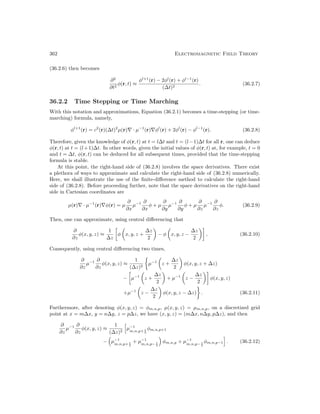
![Computational Electromagnetics, Finite Difference Method, Yee Algorithm 363
This cumbersome equation can be abbreviated if we define a central difference operator
as2
¯
∂zφm =
1
∆z
φm+ 1
2
− φm− 1
2
(36.2.13)
Then the right-hand side of the (36.2.12) can be written succinctly as
∂
∂z
µ−1 ∂
∂z
φ(x, y, z) ≈ ¯
∂zµm,n,p
¯
∂zφm,n,p (36.2.14)
With similar approximations to the other terms in (36.2.9), Equation (36.2.8) becomes
φl+1
m,n,p = (∆t)2
c2
m,n,pµm,n,p
¯
∂xµm,n,p
¯
∂x + ¯
∂yµm,n,p
¯
∂y + ¯
∂zµm,n,p
¯
∂z
φm,n,p
+ 2φl
m,n,p − φl−1
m,n,p. (36.2.15)
The above can be readily implemented on a computer for time stepping. Notice however,
that the use of central differencing results in the evaluation of medium property µ at half
grid points. This is inconvenient, as the introduction of half grid points increases computer
memory requirements. Hence, it is customary to the medium property at the integer grid
points, and to approximate
µm+ 1
2 ,n,p '
1
2
(µm+1,n,p + µm,n,p), (36.2.16)
µm+ 1
2 ,n,p + µm− 1
2 ,n,p ' 2µm,n,p, (36.2.17)
and so on. Moreover, if µ is a smooth function of space, it is easy to show that the errors in
the above approximations are of second order by Taylor series expansions.
For a homogeneous medium, with ∆x = ∆y = ∆z = ∆s, (36.2.15) becomes
φl+1
m,n,p =
∆t
∆s
2
c2
φl
m+1,n,p + φl
m−1,n,p + φl
m,n+1,p + φl
m,n−1,p + φl
m,n,p+1
+ φl
m,n,p−1 − 6φl
m,n,p
+ 2φl
m,n,p − φl−1
m,n,p. (36.2.18)
Notice then that with the central-difference approximation, the value of φl+1
m,n,p is dependent
only on φl
m,n,p, and its nearest neighbors, φl
m±1,n,p, φl
m,n±1,p, φl
m,n,p±1, and φl−1
m,n,p, its value
at the previous time step. Moreover, in the finite-difference scheme outlined above, no matrix
inversion is required at each time step. Such a scheme is also known as an explicit scheme.
The use of an explicit scheme is a major advantage of the finite-difference method compared
to the finite-element methods. Consequently, in order to update N grid points using (36.2.15)
or (36.2.18), O(N) multiplications are required for each time step. In comparison, O(N3
)
multiplications are required to invert an N × N full matrix, e.g., using Gaussian elimination.
The simplicity and efficiency of these algorithms have made them very popular.
2This is in the spirit of [202].](https://image.slidesharecdn.com/emftall20191204-240115133321-d13ecad1/85/EMFTAll2-377-320.jpg)
![364 Electromagnetic Field Theory
36.2.3 Stability Analysis
The implementation of the finite-difference scheme does not always lead to a stable scheme.
Hence, in order for the solution to converge, the time-stepping scheme must at least be stable.
Consequently, it is useful to find the condition under which a numerical finite-difference
scheme is stable. To do this, one performs the von Neumann stability analysis (von Neumann
1943 [203]) on Equation (36.2.18). We will assume the medium to be homogeneous to simplify
the analysis.
As shown previously, any wave can be expanded in terms of sum of plane waves in different
directions. So if a scheme is not stable for a plane wave, it would not be stable for any wave.
Consequently, to perform the stability analysis, we assume a propagating plane wave as a
trial solution
φ(x, y, z, t) = A(t)eikxx+ikyy+ikzz
, (36.2.19)
In discretized form, it is just
φl
m,n,p = Al
eikxm∆s+ikyn∆s+ikzp∆s
. (36.2.20)
Using (36.2.20), it is easy to show that for the x space derivative,
φl
m+1,n,p − 2φl
m,n,p + φl
m−1,n,p = 2[cos(kx∆s) − 1]φl
m,n,p
= −4 sin2
kx∆s
2
φl
m,n,p. (36.2.21)
The space derivatives in y and z directions can be similarly derived.
The time derivative can be treated and it is proportional to
∂2
∂t2
φ(r, t)(∆t)2
≈ φl+1
m,n,p − 2φl
m,n,p + φl−1
m,n,p. (36.2.22)
Substituting (36.2.20) into the above, we have the second time derivative being proportional
to
∂2
∂t2
φ(r, t)(∆t)2
≈ (Al+1
− 2Al
+ Al−1
)eikxm∆s+ikyn∆s+ikzp∆s
(36.2.23)
To simplify further, one can assume that
Al+1
= gAl
. (36.2.24)
This is commensurate with assuming that
A(t) = A0e−iωt
(36.2.25)
where ω can be complex. In other words, our trial solution (36.2.19) is also a time-harmonic
signal. If the finite-difference scheme is unstable for such a signal, it is unstable for all signals.
Consequently, the time derivative is proportional to
∂2
∂t2
φ(r, t)(∆t)2
≈ (g − 2 + g−1
)φl
m,n,p (36.2.26)](https://image.slidesharecdn.com/emftall20191204-240115133321-d13ecad1/85/EMFTAll2-378-320.jpg)
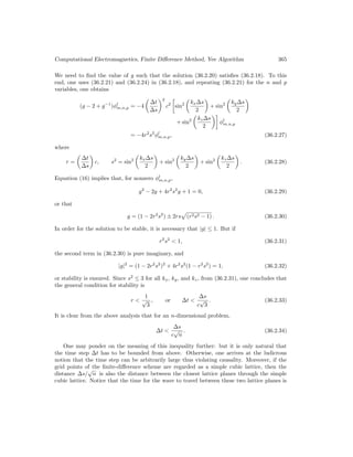
![366 Electromagnetic Field Theory
∆s/(c
√
n ). Consequently, the stability criterion (36.2.34) implies that the time step ∆t has to
be less than the shortest travel time for the wave between the lattice planes in order to satisfy
causality. In other words, if the wave is time-stepped ahead of the time on the right-hand side
of (36.2.34), instability ensues. The above is also known as the CFL (Courant, Friedrichs,
and Lewy 1928 [204]) stability criterion. It could be easily modified for ∆x 6= ∆y 6= ∆z.
The above analysis implies that we can pick a larger time step if the space steps are
larger. A larger time step will allow one to complete generating a time-domain response
rapidly. However, one cannot arbitrary make the space step large due to grid-dispersion
error, as shall be discussed next.
36.2.4 Grid-Dispersion Error
When a finite-difference scheme is stable, it still may not produce good results because of
the errors in the scheme. Hence, it is useful to ascertain the errors in terms of the size of
the grid and the time step. An easy error to analyze is the grid-dispersion error. In a
homogeneous, dispersionless medium, all plane waves propagate with the same phase velocity.
However, in the finite-difference approximation, all plane waves will not propagate at the same
phase velocity due to the grid-dispersion error.
As a consequence, a pulse in the time domain, which is a linear superposition of plane waves
with different frequencies, will be distorted if the dispersion introduced by the finite-difference
scheme is intolerable. Therefore, to make things simpler, we will analyze the grid-dispersion
error in a homogeneous free space medium.
To ascertain the grid-dispersion error, we assume the solution is time-harmonic, or that
Al
= e−iωl∆t
in (36.2.20). In this case, the left-hand side of (36.2.27) becomes
e−iω∆t
− 2 + e+iω∆t
φl
m,n,p = −4 sin2
ω∆t
2
φl
m,n,p. (36.2.35)
Then, from Equation (36.2.27), it follows that
sin
ω∆t
2
= rs, (36.2.36)
where r and s are given in (36.2.28). Now, Equation (36.2.36) governs the relationship between
ω and kx, ky, and kz in the finite-difference scheme, and hence, is a dispersion relation.
But if a medium is homogeneous, it is well known that (36.2.1) has a plane-wave solution
of the type given by (36.2.19) where
ω = c
q
k2
x + k2
y + k2
z = c|k| = ck. (36.2.37)
where k = x̂kx + ŷky + ẑkz is the direction of propagation of the plane wave. Defining the
phase velocity to be ω/k = c, this phase velocity is isotropic, or the same in all directions.
Moreover, it is independent of frequency. But in (36.2.36), because of the definition of s as
given by (36.2.28), the dispersion relation between ω and k is not isotropic. This implies that
plane waves propagating in different directions will have different phase velocities.](https://image.slidesharecdn.com/emftall20191204-240115133321-d13ecad1/85/EMFTAll2-380-320.jpg)
![Computational Electromagnetics, Finite Difference Method, Yee Algorithm 367
Equation (36.2.36) departs from Equation (36.2.37) as a consequence of the finite-difference
approximation. This departure gives rise to errors, which are the consequence of grid disper-
sion. For example, when c is a constant, (36.2.37) states that the phase velocities of plane
waves of different wavelengths and directions are the same. However, this is not true for
(36.2.36), as shall be shown.
Assuming s small, (36.2.36), after using Taylor series expansion, can be written as
ω∆t
2
= sin−1
rs ∼
= rs +
r3
s3
6
. (36.2.38)
When ∆s is small, using the small argument approximation for the sine function, one obtains
from (36.2.28)
s '
∆s
2
(k2
x + k2
y + k2
z)1/2
(36.2.39)
Equation (36.2.38), by taking the higher-order Taylor expansion of (36.2.38), then becomes
ω∆t
2
' r
∆s
2
(k2
x + k2
y + k2
z)1/2
[1 − δ] (36.2.40)
where (see [34])
δ =
∆s2
24
k4
x + k4
y + k4
z
k2
x + k2
y + k2
z
+
r2
∆s2
24
(k2
x + k2
y + k2
z) (36.2.41)
Since k is inversely proportional to wavelength λ, then δ in the correction to the above
equation is proportional to ∆s2
/λ2
. Therefore, to reduce the grid dispersion error, it is
necessary to have
∆s
λ
2
1. (36.2.42)
When this is true, using the fact that r = c∆t/∆s, then (36.2.40) becomes
ω
c
≈
q
k2
x + k2
y + k2
z . (36.2.43)
which is close to the dispersion relation of free space. Consequently, in order for the finite-
difference scheme to propagate a certain frequency content accurately, the grid size must be
much less than the wavelength of the corresponding frequency. Furthermore, ∆t must be
chosen so that the CFL stability criterion is met. Hence, the rule of thumb is to choose about
10 to 20 grid points per wavelength. Also, for a plane wave propagating as eik·r
, an error
δk in the vector k gives rise to cumulative error eiδk·r
. The larger the distance traveled, the
larger the cumulative phase error, and hence the grid size must be smaller in order to arrest
such phase error due to the grid dispersion.](https://image.slidesharecdn.com/emftall20191204-240115133321-d13ecad1/85/EMFTAll2-381-320.jpg)
![368 Electromagnetic Field Theory
36.3 The Yee Algorithm
The Yee algorithm (Yee 1966 [194]) is specially designed to solve vector electromagnetic field
problems on a rectilinear grid. The finite-difference time-domain (FDTD) method (Taflov
1988) when applied to solving electromagnetics problems, usually uses this method. To derive
it, Maxwell’s equations are first written in Cartesian coordinates:
−
∂Bx
∂t
=
∂Ez
∂y
−
∂Ey
∂z
, (36.3.1)
−
∂By
∂t
=
∂Ex
∂z
−
∂Ez
∂x
, (36.3.2)
−
∂Bz
∂t
=
∂Ey
∂x
−
∂Ex
∂y
, (36.3.3)
∂Dx
∂t
=
∂Hz
∂y
−
∂Hy
∂z
− Jx, (36.3.4)
∂Dy
∂t
=
∂Hx
∂z
−
∂Hz
∂x
− Jy, (36.3.5)
∂Dz
∂t
=
∂Hy
∂x
−
∂Hx
∂y
− Jz. (36.3.6)
Figure 36.2: The assignment of fields on a grid in the Yee algorithm.
After denoting f(n∆x, m∆y, p∆z, l∆t) = fl
m,n,p, and replacing derivatives with central
finite-differences in accordance with Figure 36.2, (36.3.1) becomes
1
∆t
B
l+ 1
2
x,m,n+ 1
2 ,p+ 1
2
− B
l− 1
2
x,m,n+ 1
2 ,p+ 1
2
=
1
∆z
El
y,m,n+ 1
2 ,p+1 − El
y,m,n+ 1
2 ,p
−
1
∆y
El
z,m,n+1,p+ 1
2
− El
z,m,n,p+ 1
2
. (36.3.7)](https://image.slidesharecdn.com/emftall20191204-240115133321-d13ecad1/85/EMFTAll2-382-320.jpg)
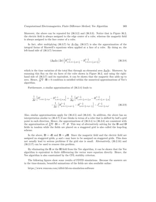
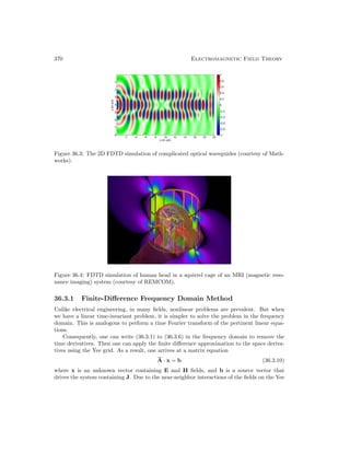
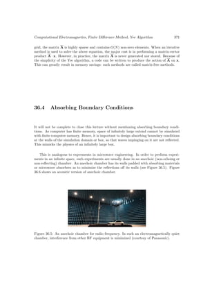
![372 Electromagnetic Field Theory
Figure 36.6: An acoustic anechoic chamber. In such a chamber, even the breast-feeding sound
of a baby can be heard clearly (courtesy of AGH University, Poland).
By the same token, in order to simulate an infinite box with a finite-size box, absorbing
boundary conditions (ABCs) are designed at its walls. The simplest of such ABCs is the
impedance boundary condition. (A transmission line terminated with an impedance reflects
less than one terminated with an open or a short circuit.) Another simple ABC is to mimick
the Sommerfeld radiation condition (much of this is reviewed in [34].
A recently invented ABC is the perfectly matched layers (PML) [205]. Also, another
similar ABC is the stretched coordinates PML [206]. Figure 36.7 shows simulation results
with and without stretched coordinates PMLs on the walls of the simulation domain [207].
Figure 36.7: Simulation of a source on top of a half-space (left) without stretched coordinates
PML; and (right) with stretched coordinats PML [207].](https://image.slidesharecdn.com/emftall20191204-240115133321-d13ecad1/85/EMFTAll2-386-320.jpg)
![374 Electromagnetic Field Theory
An example of vector differential equation for vector electromagnetic field is
∇ × µ−1
· ∇ × E(r) − ω2
· E(r) = iωJ(r) (37.1.2)
These equations are linear equations. They have one commonality, i.e., they can be
abstractly written as
L f = g (37.1.3)
where L is the differential operator which is linear, and f is the unknown, and g is the
driving source. Differential equations, or partial differential equations, as mentioned before,
have to be solved with boundary conditions. Otherwise, there is no unique solution to these
equations.
In the case of the scalar wave equation (37.1.1), L = (∇2
+ k2
) is a differential operator.
In the case of the electromagnetic vector wave equation (37.1.2), L = (∇×µ−1
·∇×)−ω2
·.
Furthermore, f will be φ(r) for the scalar wave equation (37.1.1), while it will be E(r) in the
case of vector wave equation for an electromagnetic system (37.1.2). The g on the right-hand
side can represent Q in (37.1.1) or iωJ(r) in (37.1.2).
37.1.2 Examples of Integral Equations
This course is replete with PDE’s, but we have not come across too many integral equations.
Therefore, we shall illustrate the derivation of some integral equations. Since the acoustic
wave problem is homomorphic to the electromagnetic wave problem, we will illustrate the
derivation of integral equation of scattering using acoustic wave equation.1
The surface integral equation method is rather popular in a number of applications, be-
cause it employs a homogeneous-medium Green’s function which is simple in form, and the
unknowns reside on a surface rather than in a volume. In this section, the surface integral
equations2
for scalar and will be studied first. Then, the volume integral equation will be
discussed next.
Surface Integral Equations
In an integral equation, the unknown to be sought is embedded in an integral. An integral
equation can be viewed as an operator equation as well, just as are differential equations. We
shall see how such integral equations with only surface integrals are derived, using the scalar
wave equation.
1The cases of electromagnetic wave equations can be found in Chew, Waves and Fields in Inhomogeneous
Media [34].
2These are sometimes called boundary integral equations [208,209].](https://image.slidesharecdn.com/emftall20191204-240115133321-d13ecad1/85/EMFTAll2-388-320.jpg)
![Computational Electromagnetics, Numerical Methods 375
Figure 37.1: A two-region problem can be solved with a surface integral equation.
Consider a scalar wave equation for a two-region problem as shown in Figure 37.1. In
region 1, the governing equation for the total field is
(∇2
+ k2
1) φ1(r) = Q(r), (37.1.4)
For simplicity, we will assume that the scatterer is impenetrable, meaning that the field in
region 2 is zero. Therefore, we need only define Green’s functions for regions 1 to satisfy the
following equations:
(∇2
+ k2
1) g1(r, r
) = −δ(r − r
), (37.1.5)
The derivation here is similar to the that of Huygens’ principle. On multiplying Equation
(37.1.1) by g1(r, r
) and Equation (37.1.5) by φ1(r), subtracting the two resultant equations,
and integrating over region 1, we have, for r
∈ V1,
V1
dV [g1(r, r
)∇2
φ1(r) − φ1(r)∇2
g1(r, r
)]
=
V1
dV g1(r, r
)Q(r) + φ1(r
), r
∈ V1. (37.1.6)
Since ∇ · (g∇φ − φ∇g) = g∇2
φ − φ∇2
g, by applying Gauss’ theorem, the volume integral
on the left-hand side of (37.1.6) becomes a surface integral over the surface bounding V1.
Consequently,3
−
S+Sinf
dS n̂ · [g1(r, r
)∇φ1(r) − φ1(r)∇g1(r, r
)]
= −φinc(r
) + φ1(r
), r
∈ V1. (37.1.7)
3The equality of the volume integral on the left-hand side of (37.1.6) and the surface integral on the
left-hand side of (37.1.7) is also known as Green’s theorem.](https://image.slidesharecdn.com/emftall20191204-240115133321-d13ecad1/85/EMFTAll2-389-320.jpg)
![376 Electromagnetic Field Theory
In the above, we have let
φinc(r0
) = −
V1
dV g1(r, r0
)Q(r), (37.1.8)
since it is the incident field generated by the source Q(r).
Note that up to this point, g1(r, r0
) is not explicitly specified, as long as it is a solution of
(37.1.5). A simple choice for g1(r, r0
) that satisfies the radiation condition is
g1(r, r0
) =
eik1|r−r0
|
4π|r − r0|
, (37.1.9)
It is the unbounded, homogeneous medium scalar Green’s function. In this case, φinc(r) is
the incident field generated by the source Q(r) in the absence of the scatterer. Moreover, the
integral over Sinf vanishes when Sinf → ∞ by virtue of the radiation condition. Then, after
swapping r and r0
, we have
φ1(r) = φinc(r) −
S
dS0
n̂0
· [g1(r, r0
)∇0
φ1(r0
) − φ1(r0
)∇0
g1(r, r0
)], r ∈ V1. (37.1.10)
But if r0
/
∈ V1 in (37.1.6), the second term, φ1(r), on the right-hand side of (37.1.6) would be
zero, for r0
would be in V2 where the integration is not performed. Therefore, we can write
(37.1.10) as
if r ∈ V1, φ1(r)
if r ∈ V2, 0
= φinc(r) −
S
dS0
n̂0
· [g1(r, r0
)∇0
φ1(r0
) − φ1(r0
)∇0
g1(r, r0
)]. (37.1.11)
The above equation is evocative of Huygens’ principle. It says that when the observation
point r is in V1, then the total field φ1(r) consists of the incident field, φinc(r), and the
contribution of field due to surface sources on S, which is the second term on the right-hand
side of (37.1.11). But if the observation point is in V2, then the surface sources on S generate
a field that exactly cancels the incident field φinc(r), making the total field in region 2 zero.
This fact is the core of the extinction theorem as shown in Figure 37.2 (see Born and Wolf
1980).
In (37.1.11), n̂ · ∇φ1(r) and φ1(r) act as surface sources. Moreover, they are impressed on
S, creating a field in region 2 that cancels exactly the incident field in region 2 (see Figure
37.2).](https://image.slidesharecdn.com/emftall20191204-240115133321-d13ecad1/85/EMFTAll2-390-320.jpg)
![Computational Electromagnetics, Numerical Methods 377
Figure 37.2: The illustration of the extinction theorem.
Applying the extinction theorem, integral equations can now be derived. So, using the
lower parts of Equations (37.1.11), we have
φinc(r) =
S
dS
n̂
· [g1(r, r
)∇
φ1(r
) − φ1(r
)∇
g1(r, r
)], r ∈ V2, (37.1.12)
The integral equations above still has two independent unknowns, φ1 and n̂ · ∇φ1. Next,
boundary conditions can be used to eliminate one of these two unknowns.
An acoustic scatterer which is impenetrable either has a hard surface boundary condition
where normal velocity is zero, or it has soft surface where the pressure is zero (also called a
pressure release surface). Since the force or the velocity of the particle is proportional to the
∇φ, a hard surface will have n̂ · ∇φ1 = 0, or a homogeneous Neumann boundary condition,
while a soft surface will have φ1 = 0, a homogeneous Dirichlet boundary condition.
φinc(r) =
S
dS
n̂
· [g1(r, r
)∇
φ1(r
)], r ∈ V2, soft boundary condition
(37.1.13)
φinc(r) = −
S
dS
φ1(r
)∇
g1(r, r
], r ∈ V2, hard boundary condition
(37.1.14)
More complicated surface integral equations (SIEs) for penetrable scatterers, as well as
vector surface integral equations for the electromagnetics cases are derived in Chew, Waves
and Fields in Inhomogeneous Media [34,210]. Also, there is another class of integral equations
called volume integral equations (VIEs) [211]. They are also derived in [34].
Nevertheless, all the linear integral equations can be unified under one notation:
L f = g (37.1.15)
where L is a linear operator. This is similar to the differential equation case. The difference
is that the unknown f represents the source of the problem, while g is the incident field
impinging on the scatterer or object. Furthermore, f does not need to satisfy any boundary
condition, since the field radiated via the Green’s function satisfies the radiation condition.](https://image.slidesharecdn.com/emftall20191204-240115133321-d13ecad1/85/EMFTAll2-391-320.jpg)
![380 Electromagnetic Field Theory
In the above, fn, n, . . . , N are known functions called basis functions. Now, an’s are the
new unknowns to be sought. Also the above is an approximation, and the accuracy of the
approximation depends very much on the original function f. A set of very popular basis
functions are functions that form a piece-wise linear interpolation of the function from its
nodes. These basis functions are shown in Figure 37.4.
Figure 37.4: Examples of basis function in (a) one dimension, (b) two dimension. Each of
these functions are define over a finite domain. Hence, they are also called sub-domain basis
functions.
Upon substituting (37.2.3) into (37.2.1), we obtain
N
n=1
anL fn = g (37.2.4)
Then, multiplying (37.2.4) by wm and integrate over the space that wm(r) is defined, then
we have
N
n=1
an wm, L fn = wm, g , m = 1, . . . , N (37.2.5)
In the above, the inner product is defined as
f1, f2 = drf1(r)f2(r) (37.2.6)
where the integration is over the support of the functions, or the space over which the functions
are defined.5
For PDEs these functions are defined over a 3D space, while in SIEs, these
5This is known as the reaction inner product [34,47,120]. As oppose to most math and physics literature,
the energy inner product is used [120].](https://image.slidesharecdn.com/emftall20191204-240115133321-d13ecad1/85/EMFTAll2-394-320.jpg)
![Computational Electromagnetics, Numerical Methods 381
functions are defined over a surface. In a 1D problems, these functions are defined over a 1D
space.
The functions wm, m = 1, . . . , N is known as the weighting functions or testing functions.
The testing functions should be chosen so that they can approximate well a function that
lives in the range space W of the operator L . Such set of testing functions lives in the dual
space of the range space. For example, if fr lives in the range space of the operator L , the
set of function fd, such that the inner product hfd, fri exists, forms the dual space of W.
The above is a matrix equation of the form
L · a = g (37.2.7)
where
L
mn
= hwm, L fni
[a]n = an, [g]m = hwm, gi
(37.2.8)
What has effectively happened here is that given an operator L that maps a function that lives
in an infinite dimensional Hilbert space V , to another function that lives in another infinite
dimensional Hilbert space W, via the operator equation L f = g, we have approximated
the Hilbert spaces with finite dimensional spaces (subspaces), and finally, obtain a finite
dimensional matrix equation that is the representation of the original infinite dimensional
operator equation.
In the above, L is the matrix representation of the operator L in the subspaces, and a
and g are the vector representations of f and g, respectively, in their respective subspaces.
When such a method is applied to integral equations, it is usually called the method
of moments (MOM). (Surface integral equations are also called boundary integral equations
(BIEs) in other fields [209]. When finite discrete basis are used to represent the surface
unknowns, it is also called the boundary element method (BEM) [212]. But when this method
is applied to solve PDEs, it is called the finite element method (FEM) [213–216], which is a
rather popular method due to its simplicity.
37.2.4 Mesh Generation
In order to approximate a function defined on an arbitrary shaped surface or volume by
sum of basis functions, it is best to mesh (tessellate or discretize) the surface and volume by
meshes. In 2D, all shapes can be tessellated by unions of triangles, while a 3D volume can be
meshed (tessellated) by unions of tetrahedrons. Such meshes are used not only in CEM, but
in other fields such as solid mechanics. Hence, there are many commercial software available
to generate sophisticated meshes.
When a surface is curved, or of arbitrary shape, it can be meshed by union of triangles as
shown in Figure 37.5. When a volume is of arbitrary shape of a volume is around an arbitrary
shape object, it can be meshed by tetrahedrons as shown in Figure 37.6. Then basis functions
are defined to interpolate the field between nodal values or values defined on the edges of a
triangle or a tetrahedron.](https://image.slidesharecdn.com/emftall20191204-240115133321-d13ecad1/85/EMFTAll2-395-320.jpg)
![382 Electromagnetic Field Theory
Figure 37.5: An arbitrary surface can be meshed by a union of triangles.
Figure 37.6: A volume region can be meshed by a union of tetrahedra. But the surface of the
aircraft is meshed with a union of trianlges (courtesy of gmsh.info).
37.3 Solving Matrix Equation by Optimization
When a matrix system get exceedingly large, it is preferable that a direct inversion of the
matrix equation not performed. Direct inversions (e.g., using Gaussian elimination [217]
or Kramer’s rule [218]) have computational complexity6
of O(N3
), and requiring storage of
O(N2
). Hence, when N is large, other methods have to be sought.
To this end, it is better to convert the solving of a matrix equation into an optimiza-
tion problem. These methods can be designed so that a much larger system can be solved
with a digital computer. Optimization problem results in finding the stationary point of a
functional.7
First, we will figure out how to find such a functional.
Consider a matrix equation given by
L · f = g (37.3.1)
6The scaling of computer time with respect to the number of unknowns (degrees of freedom) is known in
the computer parlance as computational complexity.
7Functional is usually defined as a function of a function [34, 43]. Here, we include a function of a vector
to be a functional as well.](https://image.slidesharecdn.com/emftall20191204-240115133321-d13ecad1/85/EMFTAll2-396-320.jpg)
![Computational Electromagnetics, Numerical Methods 383
For simplicity, we consider L as a symmetric matrix.8
Then one can define a functional
I = ft
· L · f − 2ft
· g (37.3.2)
Such a functional is called a quadratic functional because it is analogous to I = Lx2
− 2xg,
which is quadratic, in its simplest 1D rendition.
Taking the first variation with respect to f, namely, we let f = fo +δf, and find the leading
order approximation of the functional. Therefore, one gets
δI = δft
· L · fo + ft
o · L · δf − 2δft
· g (37.3.3)
If L is symmetric, the first two terms are the same, and the above becomes
δI = 2δft
· L · fo − 2δft
· g (37.3.4)
For fo to be the optimal point or the stationary point, then its first variation has to be zero,
or that δI = 0. Thus we conclude that
L · fo = g (37.3.5)
Hence, the optimal point to the functional I in (37.3.2) is the solution to (37.3.1).
Such method, when applied to an infinite dimensional Hilbert space problem, is called
variational method, but the main ideas are similar. The wonderful idea about such a method
is that instead of doing direct inversion, one can search for the optimal point or stationary
point of the quadratic functional using gradient search or gradient descent methods or some
optimization method.
37.3.1 Gradient of a Functional
It turns out that the gradient of a quadratic functional can be found quite easily. Also it
is cheaper to computer the gradient of a functional than to find the inverse of a matrix
operator. To do this, it is better to write out functional using index (or indicial, or Einstein)
notation [219]. In this notation, the functional first variation δI in (37.3.4) becomes
δI = 2δfjLijfi − 2δfjgj (37.3.6)
In the above, we neglect to distinguish between fo and f and f represents the optimal point
is implied. Also, in this notation, the summation symbol is dropped, and summations over
repeated indices are implied. In this notation, it is easier to see what a functional derivative
is. We can differentiate the above with respect to fj easily to arrive at
∂I
∂fj
= 2Lijfi − 2gj (37.3.7)
8Functional for the asymmetric case can be found in Chew, Waves and Fields in Inhomogeneous Media,
Chapter 5 [34].](https://image.slidesharecdn.com/emftall20191204-240115133321-d13ecad1/85/EMFTAll2-397-320.jpg)
![384 Electromagnetic Field Theory
Notice that the remaining equation has one index j remaining in index notation, meaning
that it is a vector equation. We can reconstitute the above using our more familiar matrix
notation that
∇f I = 2L · f − 2g (37.3.8)
The left-hand side is a notation for the gradient of a functional in a multi-dimensional space
defined by f, and the right-hand side is the expression for calculating this gradient. One needs
only to perform a matrix-vector product to find this gradient. Hence, the computational
complexity of finding this gradient is O(N2
) at worst, and O(N) for many sparse matrices.
In a gradient search method, such a gradient is calculated repeated until the optimal point is
found. Such methods are called iterative methods.
If the optimal point can be found in Niter iterations, then the CPU time scales as NiterNα
where 1 α 2. There is a clever gradient search algorithm, called the conjugate gradient
method that can find the optimal point in Niter in exact arithmetics. In many gradient search
methods, Niter N resulting in great savings in computer time.
What is more important is that this method does not require the storage of the matrix L,
but a computer code that produces the vector go = L · f as an output, with f as an input.
Both f and go require only O(N) memory storage. Such methods are called matrix-free
methods. Even when L is a dense matrix, but is the matrix representation of some Green’s
function, fast methods now exist to perform the dense matrix-vector product in O(N log N)
operations.9
The value I is also called the cost function, and its minimum is sought in the seeking of
the solution by gradient search methods. Detail discussion of these methods is given in [220].
Figure 37.7 shows the contour plot of a cost function in 2D. When the condition number10
of the matrix L is large (implying that the matrix is ill-conditioned), the contour plot will
resemble a deep valley. And hence, the gradient search method will tend to zig-zag along the
way as it finds the solution. Therefore, convergence is slow for matrices with large condition
numbers
9Chew et al, Fast and Efficient Algorithms in CEM [9].
10This is the ratio of the largest eigenvalue of the matrix to its smallest eigenvalue.](https://image.slidesharecdn.com/emftall20191204-240115133321-d13ecad1/85/EMFTAll2-398-320.jpg)
![Computational Electromagnetics, Numerical Methods 385
Figure 37.7: Plot of a 2D cost function for an ill-conditioned system (courtesy of Numerical
Recipe [220]).
Figure 37.8 shows a cartoon picture in 2D of the histories of different search paths from a
machine-learning example where a cost functional similar to I has to be minimized. Finding
the optimal point or the minimum point of a general functional is still a hot topic of research:
it is important in artificial intelligence.
Figure 37.8: Gradient search or gradient descent method is finding an optimal point (courtesy
of Y. Ioannou: https://blog.yani.io/sgd/).](https://image.slidesharecdn.com/emftall20191204-240115133321-d13ecad1/85/EMFTAll2-399-320.jpg)

![Lecture 38
Quantum Theory of Light
38.1 Quantum Theory of Light
38.1.1 Historical Background
Quantum theory is a major intellectual achievement of the twentieth century, even though
we are still discovering new knowledge in it. Several major experimental findings led to the
revelation of quantum theory or quantum mechanics of nature. In nature, we know that
many things are not infinitely divisible. Matter is not infinitely divisible as vindicated by the
atomic theory of John Dalton (1766-1844) [221]. So fluid is not infinitely divisible: as when
water is divided into smaller pieces, we will eventually arrive at water molecule, H2O, which
is the fundamental building block of water.
In turns out that electromagnetic energy is not infinitely divisible either. The electromag-
netic radiation out of a heated cavity would obey a very different spectrum if electromagnetic
energy is infinitely divisible. In order to fit experimental observation of radiation from a
heated electromagnetic cavity, Max Planck (1900s) [222] proposed that electromagnetic en-
ergy comes in packets or is quantized. Each packet of energy or a quantum of energy E is
associated with the frequency of electromagnetic wave, namely
E = ~ω = ~2πf = hf (38.1.1)
where ~ is now known as the Planck constant and ~ = h/2π = 6.626 × 10⁻³⁴
J·s (Joule-
second). Since ~ is very small, this packet of energy is very small unless ω is large. So it
is no surprise that the quantization of electromagnetic field is first associated with light, a
very high frequency electromagnetic radiation. A red-light photon at a wavelength of 700
nm corresponds to an energy of approximately 2 eV ≈ 3 × 10⁻¹⁹
J ≈ 75 kBT, where kBT
denotes the thermal energy. A microwave photon has approximately 1 × 10⁻⁵
eV.
The second experimental evidence that light is quantized is the photo-electric effect [223].
It was found that matter emitted electrons when light shined on it. First, the light frequency
has to correspond to the “resonant” frequency of the atom. Second, the number of electrons
emitted is proportional to the number of packets of energy ~ω that the light carries. This
387](https://image.slidesharecdn.com/emftall20191204-240115133321-d13ecad1/85/EMFTAll2-401-320.jpg)
![388 Electromagnetic Field Theory
was a clear indication that light energy traveled in packets or quanta as posited by Einstein
in 1905.
That light is a wave has been demonstrated by Newton’s ring effect [224] in the eighteenth
century (1717) (see Figure 38.1). In 1801, Thomas Young demonstrated the double slit
experiment [225] that further confirmed the wave nature of light (see Figure 38.2). But by
the beginning of the 20-th century, one has to accept that light is both a particle, called a
photon, carrying a quantum of energy with momentum, as well as a particle endowed with
wave-like behavior. This is called wave-particle duality.
Figure 38.1: A Newton’s rings experiment (courtesy of [224]).](https://image.slidesharecdn.com/emftall20191204-240115133321-d13ecad1/85/EMFTAll2-402-320.jpg)
![Quantum Theory of Light 389
Figure 38.2: A Young’s double-slit experiment (courtesy of [226]).
This concept was not new to quantum theory as electrons were known to behave both like
a particle and a wave. The particle nature of an electron was confirmed by the measurement
of its charge by Millikan in 1913 in his oil-drop experiment. (The double slit experiment for
electron was done in 1927 by Davison and Germer, indicating that an electron has a wave
nature [225].) In 1924, De Broglie [227] suggested that there is a wave associated with an
electron with momentum p such that
p = k (38.1.2)
where k = 2π/λ, the wavenumber. All this knowledge gave hint to the quantum theorists of
that era to come up with a new way to describe nature.
Classically, particles like an electron moves through space obeying Newton’s laws of mo-
tion first established in 1687 [228]. Old ways of describing particle motion were known as
classical mechanics, and the new way of describing particle motion is known as quantum
mechanics. Quantum mechanics is very much motivated by a branch of classical mechanics
called Hamiltonian mechanics. We will first use Hamiltonian mechanics to study a simple
pendulum and connect it with electromagnetic oscillations.
38.1.2 Connecting Electromagnetic Oscillation to Simple Pendulum
The quantization of electromagnetic field theory was started by Dirac in 1927 [3]. In the be-
ginning, it was called quantum electrodynamics important for understanding particle physics](https://image.slidesharecdn.com/emftall20191204-240115133321-d13ecad1/85/EMFTAll2-403-320.jpg)
![390 Electromagnetic Field Theory
phenomena and light-matter interactions [229]. Later on, it became important in quantum
optics where quantum effects in electromagnetics technologies first emerged. Now, microwave
photons are measurable and are important in quantum computers. Hence, quantum effects
are important in the microwave regime as well.
Maxwell’s equations can be regarded as for describing an infinite set of coupled harmonic
oscillators. In one dimension, when a wave propagates on a string, or an electromagnetic
wave propagating on a transmission line, they can be regarded as propagating on a set of
coupled harmonic oscillators as shown in Figure 38.3. Maxwell’s equations describe the waves
travelling in 3D space due to the coupling between an infinite set of harmonic oscillators.
In fact, methods have been developed to solve Maxwell’s equations using transmission-line-
matrix (TLM) method [230], or the partial element equivalent circuit (PEEC) method [231].
Figure 38.3: Maxwell’s equations describe the coupling of harmonic oscillators in a 3D space.
This is similar to waves propagating on a string or a 1D transmission line, or a 2D array of
coupled oscillators. The saw-tooth symbol in the figure represents a spring.
The cavity modes in electromagnetics are similar to the oscillation of a pendulum. To
understand the quantization of electromagnetic field, we start by connecting these cavity
modes oscillations to the oscillations of a simple pendulum. It is to be noted that funda-
mentally, electromagnetic oscillation exists because of displacement current. Displacement
current exists even in vacuum because vacuum is polarizable, namely that D = εE. Further-
more, displacement current exists because of the ∂D/∂t term in the generalized Ampere’s
law added by Maxwell, namely,
∇ × H =
∂D
∂t
+ J (38.1.3)](https://image.slidesharecdn.com/emftall20191204-240115133321-d13ecad1/85/EMFTAll2-404-320.jpg)
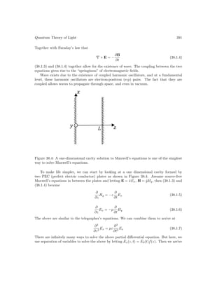
![Quantum Theory of Light 393
What is more important is that the resonance of each of these modes is similar or ho-
momorphic to the resonance of a simple pendulum or a simple harmonic oscillator. For a
fixed point in space, the field due to this oscillation is similar to the oscillation of a simple
pendulum.
As we have seen in the Drude-Lorentz-Sommerfeld mode, for a particle of mass m attached
to a spring connected to a wall, where the restoring force is like Hooke’s law, the equation of
motion of a pendulum by Newton’s law is
m
d2
x
dt2
+ κx = 0 (38.1.14)
where κ is the spring constant, and we assume that the oscillator is not driven by an external
force, but is in natural or free oscillation. By letting1
x = x0e−iωt
(38.1.15)
the above becomes
−mω2
x0 + κx0 = 0 (38.1.16)
Again, a non-trivial solution is possible only at the resonant frequency of the oscillator or
that when ω = ω0 where
ω0 =
r
κ
m
(38.1.17)
38.2 Hamiltonian Mechanics
Equation (38.1.14) can be derived by Newton’s law but it can also be derived via Hamiltonian
mechanics. Since Hamiltonian mechanics motivates quantum mechanics, we will look at the
Hamiltonian mechanics view of the equation of motion (EOM) of a simple pendulum given
by (38.1.14).
Hamiltonian mechanics, developed by Hamilton (1805-1865) [232], is motivated by energy
conservation. The Hamiltonian H of a system is given by its total energy, namely that
H = T + V (38.2.1)
where T is the kinetic energy and V is the potential energy of the system.
For a simple pendulum, the kinetic energy is given by
T =
1
2
mv2
=
1
2m
m2
v2
=
p2
2m
(38.2.2)
where p = mv is the momentum of the particle. The potential energy, assuming that the
particle is attached to a spring with spring constant κ, is given by
V =
1
2
κx2
=
1
2
mω2
0x2
(38.2.3)
1For this part of the lecture, we will switch to using exp(−iωt) time convention as is commonly used in
optics and physics literatures.](https://image.slidesharecdn.com/emftall20191204-240115133321-d13ecad1/85/EMFTAll2-407-320.jpg)
![394 Electromagnetic Field Theory
Hence, the Hamiltonian is given by
H = T + V =
p2
2m
+
1
2
mω2
0x2
(38.2.4)
At any instant of time t, we assume that p(t) = mv(t) = m d
dt x(t) is independent of x(t).2
In other words, they can vary independently of each other. But p(t) and x(t) have to time
evolve to conserve energy to keep H, the total energy, constant or independent of time. In
other words,
d
dt
H [p(t), x(t)] = 0 =
dp
dt
∂H
∂p
+
dx
dt
∂H
∂x
(38.2.5)
Therefore, the Hamilton equations of motion are derived to be3
dp
dt
= −
∂H
∂x
,
dx
dt
=
∂H
∂p
(38.2.6)
From (38.2.4), we gather that
∂H
∂x
= mω2
0x,
∂H
∂p
=
p
m
(38.2.7)
Applying (38.2.6), we have4
dx
dt
=
p
m
,
dp
dt
= −mω2
0x (38.2.8)
Combining the two equations in (38.2.8) above, we have
m
d2
x
dt2
= −mω2
0x = −κx (38.2.9)
which is also derivable by Newton’s law.
A typical harmonic oscillator solution to (38.2.9) is
x(t) = x0 cos(ω0t + ψ) (38.2.10)
The corresponding p(t) = mdx
dt is
p(t) = −mx0ω0 sin(ω0t + ψ) (38.2.11)
Hence
H =
1
2
mω2
0x2
0 sin2
(ω0t + ψ) +
1
2
mω2
0x2
0 cos2
(ω0t + ψ)
=
1
2
mω2
0x2
0 = E (38.2.12)
And the total energy E very much depends on the amplitude x0 of the oscillation.
2p(t) and x(t) are termed conjugate variables in many textbooks.
3Note that the Hamilton equations are determined to within a multiplicative constant, because one has
not stipulated the connection between space and time, or we have not calibrated our clock [233].
4We can also calibrate our clock here so that it agrees with our definition of momentum in the ensuing
equation.](https://image.slidesharecdn.com/emftall20191204-240115133321-d13ecad1/85/EMFTAll2-408-320.jpg)
![Quantum Theory of Light 395
38.3 Schrodinger Equation (1925)
Having seen the Hamiltonian mechanics for describing a simple pendulum which is homomor-
phic to a cavity resonator, we shall next see the quantum mechanics description of the same
simple pendulum: In other words, we will look at a quantum pendulum. To this end, we will
invoke Schrodinger equation.
Schrodinger equation cannot be derived just as in the case Maxwell’s equations. It is
a wonderful result of a postulate and a guessing game based on experimental observations
[63,64],. Hamiltonian mechanics says that
H =
p2
2m
+
1
2
mω2
0x2
= E (38.3.1)
where E is the total energy of the oscillator, or pendulum. In classical mechanics, the position
x of the particle associated with the pendulum is known with great certainty. But in the
quantum world, this position x of the quantum particle is uncertain and is fuzzy.
To build this uncertainty into a quantum harmonic oscillator, we have to look at it from
the quantum world. The position of the particle is described by a wave function,5
which
makes the location of the particle uncertain. To this end, Schrodinger proposed his equation
which is a partial differential equation. He was very much motivated by the experimental
revelation then that p = ~k from De Broglie and that E = ~ω from Planck’s law. Equation
(38.3.1) can be written more suggestively as
~2
k2
2m
+
1
2
mω2
0x2
= ~ω (38.3.2)
To add more depth to the above equation, one lets the above become an operator equation
that operates on a wave function ψ(x, t) so that
−
~2
2m
∂2
∂x2
ψ(x, t) +
1
2
mω2
0x2
ψ(x, t) = i~
∂
∂t
ψ(x, t) (38.3.3)
If the wave function is of the form
ψ(x, t) ∼ eikx−iωt
(38.3.4)
then upon substituting (38.3.4) into (38.3.3), we retrieve (38.3.2).
Equation (38.3.3) is Schrodinger equation in one dimension for the quantum version of
the simple harmonic oscillator. In Schrodinger equation, we can further posit that the wave
function has the general form
ψ(x, t) = eikx−iωt
A(x, t) (38.3.5)
where A(x, t) is a slowly varying function of x and t, compared to eikx−iωt
.6
In other words,
this is the expression for a wave packet. With this wave packet, the ∂2
/∂x2
can be again
5Since a function is equivalent to a vector, and this wave function describes the state of the quantum
system, this is also called a state vector.
6This is similar in spirit when we study high frequency solutions of Maxwell’s equations and paraxial wave
approximation.](https://image.slidesharecdn.com/emftall20191204-240115133321-d13ecad1/85/EMFTAll2-409-320.jpg)
![396 Electromagnetic Field Theory
approximated by −k2
as has been done in the paraxial wave approximation. Furthermore, if
the signal is assumed to be quasi-monochromatic, then i~∂/∂tψ(x, t) ≈ ~ω, we again retrieve
the classical equation in (38.3.2) from (38.3.3). Hence, the classical equation (38.3.2) is a
short wavelength, monochromatic approximation of Schrodinger equation. However, as we
shall see, the solutions to Schrodinger equation are not limited to just wave packets described
by (38.3.5).
For this course, we need only to study the one-dimensional Schrodinger equation. The
above can be converted into eigenvalue problem, just as in waveguide and cavity problems,
using separation of variables, by letting7
ψ(x, t) = ψn(x)e−iωnt
(38.3.6)
By so doing, (38.3.3) becomes
−
~2
2m
d2
dx2
+
1
2
mω2
0x2
ψn(x) = Enψn(x) (38.3.7)
where En = ~ωn is the eigenvalue of the problem while ψn(x) is the eigenfunction.
The parabolic x2
potential profile is also known as a potential well as it can provide the
restoring force to keep the particle bound to the well classically. The above equation is also
similar to the electromagnetic equation for a dielectric slab waveguide, where the second term
is a dielectric profile (mind you, varying in the x direction) that can trap a waveguide mode.
Therefore, the potential well is a trap for the particle both in classical mechanics or wave
physics.
The above equation (38.3.7) can be solved in closed form in terms of Hermite-Gaussian
functions (1864) [234], or that
ψn(x) =
s
1
2nn!
r
mω0
π~
e−
mω0
2~ x2
Hn
r
mω0
~
x
(38.3.8)
where Hn(y) is a Hermite polynomial, and the eigenvalues are
En =
n +
1
2
~ω0 (38.3.9)
Here, the eigenfunction or eigenstate ψn(x) is known as the photon number state (or just
a number state) of the solution. It corresponds to having n photons in the oscillation. If
this is conceived as the collective oscillation of the e-p pairs in a cavity, there are n photons
corresponding to energy of n~ω0 embedded in the collective oscillation. The larger En is,
the larger the number of photons there is. However, there is a curious mode at n = 0. This
corresponds to no photon, and yet, there is a wave function ψ0(x). This is the zero-point
energy state. This state is there even if the system is at its lowest energy state.
It is to be noted that in the quantum world, the position x of the pendulum is random.
Moreover, this position x(t) is mapped to the amplitude E0(t) of the field. Hence, it is the
7Mind you, the following is ωn, not ω0.](https://image.slidesharecdn.com/emftall20191204-240115133321-d13ecad1/85/EMFTAll2-410-320.jpg)
![Quantum Theory of Light 397
amplitude of an electromagnetic oscillation that becomes uncertain and fuzzy as shown in
Figure 38.5.
Figure 38.5: Schematic representation of the randomness of measured electric field. The elec-
tric field amplitude maps to the displacement (position) of the quantum harmonic oscillator,
which is a random variable (courtesy of Kira and Koch [235]).](https://image.slidesharecdn.com/emftall20191204-240115133321-d13ecad1/85/EMFTAll2-411-320.jpg)
![398 Electromagnetic Field Theory
Figure 38.6: Plots of the eigensolutions of the quantum harmonic oscillator (courtesy of
Wiki [236]).
38.4 Some Quantum Interpretations–A Preview
Schrodinger used this equation with resounding success. He derived a three-dimensional ver-
sion of this to study the wave function and eigenvalues of a hydrogen atom. These eigenvalues
En for a hydrogen atom agreed well with experimental observations that had eluded scientists
for decades. Schrodinger did not actually understand what this wave function meant. It was
Max Born (1926) who gave a physical interpretation of this wave function.
Given a wave function ψ(x, t), then |ψ(x, t)|2
∆x is the probability of finding the particle
in the interval [x, x + ∆x]. Therefore, |ψ(x, t)|2
is a probability density function (PDF), and
it is necessary that
∞
−∞
dx|ψ(x, t)|2
= 1 (38.4.1)
The position x of the particle is uncertain and is now a random variable. The average value
or expectation value of x is given by
∞
−∞
dxx|ψ(x, t)|2
= x(t) = x̄(t) (38.4.2)
This is not the most ideal notation, since although x is not a function of time, its expectation
value with respect to a time-varying function, ψ(x, t), can be time-varying.](https://image.slidesharecdn.com/emftall20191204-240115133321-d13ecad1/85/EMFTAll2-412-320.jpg)
![Quantum Theory of Light 399
Notice that in going from (38.3.1) to (38.3.3), or from a classical picture to a quantum
picture, we have let the momentum become p, originally a scalar number in the classical
world, become a differential operator, namely that
p → p̂ = −i~
∂
∂x
(38.4.3)
The momentum of a particle also becomes uncertain, and its expectation value is given by
∞
∞
dxψ∗
(x, t)p̂ψ(x, t) = −i~
∞
−∞
dxψ∗
(x, t)
∂
∂x
ψ(x, t) = hp̂(t)i = p̄(t) (38.4.4)
The expectation values of position x and the momentum operator p̂ are measurable in the
laboratory. Hence, they are also called observables.
One more very important aspect of quantum theory is that since p → p̂ = −i~ ∂
∂x , p̂ and
x do not commute. In other words, it can be shown that
[p̂, x] =
−i~
∂
∂x
, x
= −i~ (38.4.5)
In the classical world, [p, x] = 0, but not in the quantum world. In the equation above, we
can elevate x to become an operator by letting x̂ = xˆ
I, where ˆ
I is the identity operator. Then
both p̂ and x̂ are now operators, and are on the same footing. In this manner, we can rewrite
equation (38.4.5) above as
[p̂, x̂] = −i~ˆ
I (38.4.6)
It can be shown easily that when two operators share the same set of eigenfunctions,
they commute. When two operators p̂ and x̂ do not commute, it means that the expectation
values of quantities associated with the operators, hp̂i and hx̂i, cannot be determined to
arbitrary precision simultaneously. For instance, p̂ and x̂ correspond to random variables,
then the standard deviation of their measurable values, or their expectation values, obey the
uncertainty principle relationship that8
∆p∆x ≥ ~/2 (38.4.7)
where ∆p and ∆x are the standard deviation of the random variables p and x.
38.5 Bizarre Nature of the Photon Number States
The photon number states are successful in predicting that the collective e-p oscillations are
associated with n photons embedded in the energy of the oscillating modes. However, these
number states are bizarre: The expectation values of the position of the quantum pendulum
associated these states are always zero. To illustrate further, we form the wave function with
a photon-number state
ψ(x, t) = ψn(x)e−iωnt
8The proof of this is quite straightforward but is outside the scope of this course.](https://image.slidesharecdn.com/emftall20191204-240115133321-d13ecad1/85/EMFTAll2-413-320.jpg)
![Lecture 39
Quantum Coherent State of
Light
39.1 Quantum Coherent State of Light
We have seen that a photon number states1
of a quantum pendulum do not have a classical
correspondence as the average or expectation values of the position and momentum of the
pendulum are always zero for all time for this state. Therefore, we have to seek a time-
dependent quantum state that has the classical equivalence of a pendulum. This is the
coherent state, which is the contribution of many researchers, most notably, George Sudarshan
(1931–2018) [237] and Roy Glauber (1925–2018) [238] in 1963. Glauber was awarded the
Nobel prize in 2005.
We like to emphasize again that the modes of an electromagnetic cavity oscillation are
homomorphic to the oscillation of classical pendulum. Hence, we first connect the oscillation
of a quantum pendulum to a classical pendulum. Then we can connect the oscillation of
a quantum electromagnetic mode to the classical electromagnetic mode and then to the
quantum pendulum.
39.1.1 Quantum Harmonic Oscillator Revisited
To this end, we revisit the quantum harmonic oscillator or the quantum pendulum with more
mathematical depth. Rewriting Schrödinger equation as the eigenequation for the photon
number state for the quantum harmonic oscillator, we have
Ĥψn(x) =
−
~2
2m
d2
dx2
+
1
2
mω2
0x2
ψn(x) = Enψn(x). (39.1.1)
where ψn(x) is the eigenfunction, and En is the eigenvalue. The above can be changed into
a dimensionless form first by dividing ~ω0, and then let ξ =
pmω0
~ x be a dimensionless
1In quantum theory, a “state” is synonymous with a state vector or a function.
401](https://image.slidesharecdn.com/emftall20191204-240115133321-d13ecad1/85/EMFTAll2-415-320.jpg)
![408 Electromagnetic Field Theory
We can relate â†
and â, which are non-hermitian, to the momentum operator π̂ and position
operator ˆ
ξ previously defined which are hermitian. Then
â†
=
1
√
2
−iπ̂ + ˆ
ξ
(39.4.3)
â =
1
√
2
iπ̂ + ˆ
ξ
(39.4.4)
We also notice that
ˆ
ξ =
1
√
2
â†
+ â
= ξ ˆ
I (39.4.5)
π̂ =
i
√
2
â†
− â
= −i
d
dξ
(39.4.6)
Notice that both ˆ
ξ and π̂ are Hermitian operators in the above, with real expectation values.
With this, the average or expectation value of the position of the pendulum in normalized
coordinate, ξ, can be found by taking expectation with respect to the coherent state, or
hα|ˆ
ξ|αi =
1
√
2
hα|â†
+ â|αi (39.4.7)
Since by taking the complex conjugation transpose of (39.3.1)8
hα|â†
= hα|α∗
(39.4.8)
and (39.4.7) becomes
¯
ξ = hˆ
ξi = hα|ˆ
ξ|αi =
1
√
2
(α∗
+ α) hα|αi =
√
2e[α] 6= 0 (39.4.9)
Repeating the exercise for time-dependent case, when we let α → α̃(t) = αe−iω0t
, then,
letting α = |α|e−iψ
, then
hˆ
ξ(t)i =
√
2|α| cos(ω0t + ψ) (39.4.10)
By the same token,
π̄ = hπ̂i = hα|π̂|αi =
i
√
2
(α∗
− α) hα|αi =
√
2=m[α] 6= 0 (39.4.11)
For the time-dependent case, we let α → α̃(t) = αe−iω0t
,
hπ̂(t)i = −
√
2|α| sin(ω0t + ψ) (39.4.12)
Hence, we see that the expectation values of the normalized coordinate and momentum just
behave like a classical pendulum. There is however a marked difference: These values have
8Dirac notation is homomorphic with matrix algebra notation. (a · x)† = x† · (a)†.](https://image.slidesharecdn.com/emftall20191204-240115133321-d13ecad1/85/EMFTAll2-422-320.jpg)
![Quantum Coherent State of Light 409
standard deviations or variances that are non-zero. Thus, they have quantum fluctuation or
quantum noise associated with them. Since the quantum pendulum is homomorphic with the
oscillation of a quantum electromagnetic mode, the amplitude of a quantum electromagnetic
mode will have a mean and a fluctuation as well.
Figure 39.1: The time evolution of the coherent state. It follows the motion of a classical
pendulum or harmonic oscillator (courtesy of Gerry and Knight [239]).
.
Figure 39.2: The time evolution of the coherent state for different α’s. The left figure is for
α = 5 while the right figure is for α = 10. Recall that N = |α|2
.
.](https://image.slidesharecdn.com/emftall20191204-240115133321-d13ecad1/85/EMFTAll2-423-320.jpg)
![Bibliography
[1] J. A. Kong, Theory of electromagnetic waves. New York, Wiley-Interscience, 1975.
[2] A. Einstein et al., “On the electrodynamics of moving bodies,” Annalen der Physik,
vol. 17, no. 891, p. 50, 1905.
[3] P. A. M. Dirac, “The quantum theory of the emission and absorption of radiation,” Pro-
ceedings of the Royal Society of London. Series A, Containing Papers of a Mathematical
and Physical Character, vol. 114, no. 767, pp. 243–265, 1927.
[4] R. J. Glauber, “Coherent and incoherent states of the radiation field,” Physical Review,
vol. 131, no. 6, p. 2766, 1963.
[5] C.-N. Yang and R. L. Mills, “Conservation of isotopic spin and isotopic gauge invari-
ance,” Physical review, vol. 96, no. 1, p. 191, 1954.
[6] G. t’Hooft, 50 years of Yang-Mills theory. World Scientific, 2005.
[7] C. W. Misner, K. S. Thorne, and J. A. Wheeler, Gravitation. Princeton University
Press, 2017.
[8] F. Teixeira and W. C. Chew, “Differential forms, metrics, and the reflectionless absorp-
tion of electromagnetic waves,” Journal of Electromagnetic Waves and Applications,
vol. 13, no. 5, pp. 665–686, 1999.
[9] W. C. Chew, E. Michielssen, J.-M. Jin, and J. Song, Fast and efficient algorithms in
computational electromagnetics. Artech House, Inc., 2001.
[10] A. Volta, “On the electricity excited by the mere contact of conducting substances
of different kinds. in a letter from Mr. Alexander Volta, FRS Professor of Natural
Philosophy in the University of Pavia, to the Rt. Hon. Sir Joseph Banks, Bart. KBPR
S,” Philosophical transactions of the Royal Society of London, no. 90, pp. 403–431, 1800.
[11] A.-M. Ampère, Exposé méthodique des phénomènes électro-dynamiques, et des lois de
ces phénomènes. Bachelier, 1823.
[12] ——, Mémoire sur la théorie mathématique des phénomènes électro-dynamiques unique-
ment déduite de l’expérience: dans lequel se trouvent réunis les Mémoires que M.
Ampère a communiqués à l’Académie royale des Sciences, dans les séances des 4 et
413](https://image.slidesharecdn.com/emftall20191204-240115133321-d13ecad1/85/EMFTAll2-427-320.jpg)
![414 Electromagnetic Field Theory
26 décembre 1820, 10 juin 1822, 22 décembre 1823, 12 septembre et 21 novembre 1825.
Bachelier, 1825.
[13] B. Jones and M. Faraday, The life and letters of Faraday. Cambridge University Press,
2010, vol. 2.
[14] G. Kirchhoff, “Ueber die auflösung der gleichungen, auf welche man bei der unter-
suchung der linearen vertheilung galvanischer ströme geführt wird,” Annalen der Physik,
vol. 148, no. 12, pp. 497–508, 1847.
[15] L. Weinberg, “Kirchhoff’s’ third and fourth laws’,” IRE Transactions on Circuit Theory,
vol. 5, no. 1, pp. 8–30, 1958.
[16] T. Standage, The Victorian Internet: The remarkable story of the telegraph and the
nineteenth century’s online pioneers. Phoenix, 1998.
[17] J. C. Maxwell, “A dynamical theory of the electromagnetic field,” Philosophical trans-
actions of the Royal Society of London, no. 155, pp. 459–512, 1865.
[18] H. Hertz, “On the finite velocity of propagation of electromagnetic actions,” Electric
Waves, vol. 110, 1888.
[19] M. Romer and I. B. Cohen, “Roemer and the first determination of the velocity of light
(1676),” Isis, vol. 31, no. 2, pp. 327–379, 1940.
[20] A. Arons and M. Peppard, “Einstein’s proposal of the photon concept–a translation of
the Annalen der Physik paper of 1905,” American Journal of Physics, vol. 33, no. 5,
pp. 367–374, 1965.
[21] A. Pais, “Einstein and the quantum theory,” Reviews of Modern Physics, vol. 51, no. 4,
p. 863, 1979.
[22] M. Planck, “On the law of distribution of energy in the normal spectrum,” Annalen der
physik, vol. 4, no. 553, p. 1, 1901.
[23] Z. Peng, S. De Graaf, J. Tsai, and O. Astafiev, “Tuneable on-demand single-photon
source in the microwave range,” Nature communications, vol. 7, p. 12588, 2016.
[24] B. D. Gates, Q. Xu, M. Stewart, D. Ryan, C. G. Willson, and G. M. Whitesides, “New
approaches to nanofabrication: molding, printing, and other techniques,” Chemical
reviews, vol. 105, no. 4, pp. 1171–1196, 2005.
[25] J. S. Bell, “The debate on the significance of his contributions to the foundations of
quantum mechanics, Bells Theorem and the Foundations of Modern Physics (A. van
der Merwe, F. Selleri, and G. Tarozzi, eds.),” 1992.
[26] D. J. Griffiths and D. F. Schroeter, Introduction to quantum mechanics. Cambridge
University Press, 2018.
[27] C. Pickover, Archimedes to Hawking: Laws of science and the great minds behind them.
Oxford University Press, 2008.](https://image.slidesharecdn.com/emftall20191204-240115133321-d13ecad1/85/EMFTAll2-428-320.jpg)
![Quantum Coherent State of Light 415
[28] R. Resnick, J. Walker, and D. Halliday, Fundamentals of physics. John Wiley, 1988.
[29] S. Ramo, J. R. Whinnery, and T. Duzer van, Fields and waves in communication
electronics, Third Edition. John Wiley Sons, Inc., 1995, also 1965, 1984.
[30] J. L. De Lagrange, “Recherches d’arithmétique,” Nouveaux Mémoires de l’Académie de
Berlin, 1773.
[31] J. A. Kong, Electromagnetic Wave Theory. EMW Publishing, 2008, also 1985.
[32] H. M. Schey, Div, grad, curl, and all that: an informal text on vector calculus. WW
Norton New York, 2005.
[33] R. P. Feynman, R. B. Leighton, and M. Sands, The Feynman lectures on physics, Vols.
I, II, III: The new millennium edition. Basic books, 2011, also 1963, 2006, vol. 1,2,3.
[34] W. C. Chew, Waves and fields in inhomogeneous media. IEEE Press, 1995, also 1990.
[35] V. J. Katz, “The history of Stokes’ theorem,” Mathematics Magazine, vol. 52, no. 3,
pp. 146–156, 1979.
[36] W. K. Panofsky and M. Phillips, Classical electricity and magnetism. Courier Corpo-
ration, 2005.
[37] T. Lancaster and S. J. Blundell, Quantum field theory for the gifted amateur. OUP
Oxford, 2014.
[38] W. C. Chew, “Fields and waves: Lecture notes for ECE 350 at UIUC,”
https://engineering.purdue.edu/wcchew/ece350.html, 1990.
[39] C. M. Bender and S. A. Orszag, Advanced mathematical methods for scientists and
engineers I: Asymptotic methods and perturbation theory. Springer Science Business
Media, 2013.
[40] J. M. Crowley, Fundamentals of applied electrostatics. Krieger Publishing Company,
1986.
[41] C. Balanis, Advanced Engineering Electromagnetics. Hoboken, NJ, USA: Wiley, 2012.
[42] J. D. Jackson, Classical electrodynamics. John Wiley Sons, 1999.
[43] R. Courant and D. Hilbert, Methods of Mathematical Physics, Volumes 1 and 2. In-
terscience Publ., 1962.
[44] L. Esaki and R. Tsu, “Superlattice and negative differential conductivity in semicon-
ductors,” IBM Journal of Research and Development, vol. 14, no. 1, pp. 61–65, 1970.
[45] E. Kudeki and D. C. Munson, Analog Signals and Systems. Upper Saddle River, NJ,
USA: Pearson Prentice Hall, 2009.
[46] A. V. Oppenheim and R. W. Schafer, Discrete-time signal processing. Pearson Edu-
cation, 2014.](https://image.slidesharecdn.com/emftall20191204-240115133321-d13ecad1/85/EMFTAll2-429-320.jpg)
![416 Electromagnetic Field Theory
[47] R. F. Harrington, Time-harmonic electromagnetic fields. McGraw-Hill, 1961.
[48] E. C. Jordan and K. G. Balmain, Electromagnetic waves and radiating systems.
Prentice-Hall, 1968.
[49] G. Agarwal, D. Pattanayak, and E. Wolf, “Electromagnetic fields in spatially dispersive
media,” Physical Review B, vol. 10, no. 4, p. 1447, 1974.
[50] S. L. Chuang, Physics of photonic devices. John Wiley Sons, 2012, vol. 80.
[51] B. E. Saleh and M. C. Teich, Fundamentals of photonics. John Wiley Sons, 2019.
[52] M. Born and E. Wolf, Principles of optics: electromagnetic theory of propagation, in-
terference and diffraction of light. Elsevier, 2013, also 1959 to 1986.
[53] R. W. Boyd, Nonlinear optics. Elsevier, 2003.
[54] Y.-R. Shen, The principles of nonlinear optics. New York, Wiley-Interscience, 1984.
[55] N. Bloembergen, Nonlinear optics. World Scientific, 1996.
[56] P. C. Krause, O. Wasynczuk, and S. D. Sudhoff, Analysis of electric machinery.
McGraw-Hill New York, 1986.
[57] A. E. Fitzgerald, C. Kingsley, S. D. Umans, and B. James, Electric machinery.
McGraw-Hill New York, 2003, vol. 5.
[58] M. A. Brown and R. C. Semelka, MRI.: Basic Principles and Applications. John
Wiley Sons, 2011.
[59] C. A. Balanis, Advanced engineering electromagnetics. John Wiley Sons, 1999, also
1989.
[60] Wikipedia, “Lorentz force,” https://en.wikipedia.org/wiki/Lorentz force/, accessed:
2019-09-06.
[61] R. O. Dendy, Plasma physics: an introductory course. Cambridge University Press,
1995.
[62] P. Sen and W. C. Chew, “The frequency dependent dielectric and conductivity response
of sedimentary rocks,” Journal of microwave power, vol. 18, no. 1, pp. 95–105, 1983.
[63] D. A. Miller, Quantum Mechanics for Scientists and Engineers. Cambridge, UK:
Cambridge University Press, 2008.
[64] W. C. Chew, “Quantum mechanics made simple: Lecture notes for ECE 487 at UIUC,”
http://wcchew.ece.illinois.edu/chew/course/QMAll20161206.pdf, 2016.
[65] B. G. Streetman and S. Banerjee, Solid state electronic devices. Prentice hall Englewood
Cliffs, NJ, 1995.](https://image.slidesharecdn.com/emftall20191204-240115133321-d13ecad1/85/EMFTAll2-430-320.jpg)
![Quantum Coherent State of Light 417
[66] Smithsonian, “This 1600-year-old goblet shows that the romans were
nanotechnology pioneers,” https://www.smithsonianmag.com/history/
this-1600-year-old-goblet-shows-that-the-romans-were-nanotechnology-pioneers-787224/,
accessed: 2019-09-06.
[67] K. G. Budden, Radio waves in the ionosphere. Cambridge University Press, 2009.
[68] R. Fitzpatrick, Plasma physics: an introduction. CRC Press, 2014.
[69] G. Strang, Introduction to linear algebra. Wellesley-Cambridge Press Wellesley, MA,
1993, vol. 3.
[70] K. C. Yeh and C.-H. Liu, “Radio wave scintillations in the ionosphere,” Proceedings of
the IEEE, vol. 70, no. 4, pp. 324–360, 1982.
[71] J. Kraus, Electromagnetics. McGraw-Hill, 1984, also 1953, 1973, 1981.
[72] Wikipedia, “Circular polarization,” https://en.wikipedia.org/wiki/Circular
polarization.
[73] Q. Zhan, “Cylindrical vector beams: from mathematical concepts to applications,”
Advances in Optics and Photonics, vol. 1, no. 1, pp. 1–57, 2009.
[74] H. Haus, Electromagnetic Noise and Quantum Optical Measurements, ser. Advanced
Texts in Physics. Springer Berlin Heidelberg, 2000.
[75] W. C. Chew, “Lectures on theory of microwave and optical waveguides, for ECE 531
at UIUC,” https://engineering.purdue.edu/wcchew/course/tgwAll20160215.pdf, 2016.
[76] L. Brillouin, Wave propagation and group velocity. Academic Press, 1960.
[77] R. Plonsey and R. E. Collin, Principles and applications of electromagnetic fields.
McGraw-Hill, 1961.
[78] M. N. Sadiku, Elements of electromagnetics. Oxford University Press, 2014.
[79] A. Wadhwa, A. L. Dal, and N. Malhotra, “Transmission media,” https://www.
slideshare.net/abhishekwadhwa786/transmission-media-9416228.
[80] P. H. Smith, “Transmission line calculator,” Electronics, vol. 12, no. 1, pp. 29–31, 1939.
[81] F. B. Hildebrand, Advanced calculus for applications. Prentice-Hall, 1962.
[82] J. Schutt-Aine, “Experiment02-coaxial transmission line measurement using slotted
line,” http://emlab.uiuc.edu/ece451/ECE451Lab02.pdf.
[83] D. M. Pozar, E. J. K. Knapp, and J. B. Mead, “ECE 584 microwave engineering labora-
tory notebook,” http://www.ecs.umass.edu/ece/ece584/ECE584 lab manual.pdf, 2004.
[84] R. E. Collin, Field theory of guided waves. McGraw-Hill, 1960.](https://image.slidesharecdn.com/emftall20191204-240115133321-d13ecad1/85/EMFTAll2-431-320.jpg)
![418 Electromagnetic Field Theory
[85] Q. S. Liu, S. Sun, and W. C. Chew, “A potential-based integral equation method for
low-frequency electromagnetic problems,” IEEE Transactions on Antennas and Propa-
gation, vol. 66, no. 3, pp. 1413–1426, 2018.
[86] Wikipedia, “Snell’s law,” https://en.wikipedia.org/wiki/Snell’s law.
[87] G. Tyras, Radiation and propagation of electromagnetic waves. Academic Press, 1969.
[88] L. Brekhovskikh, Waves in layered media. Academic Press, 1980.
[89] Scholarpedia, “Goos-hanchen effect,” http://www.scholarpedia.org/article/
Goos-Hanchen effect.
[90] K. Kao and G. A. Hockham, “Dielectric-fibre surface waveguides for optical frequen-
cies,” in Proceedings of the Institution of Electrical Engineers, vol. 113, no. 7. IET,
1966, pp. 1151–1158.
[91] E. Glytsis, “Slab waveguide fundamentals,” http://users.ntua.gr/eglytsis/IO/Slab
Waveguides p.pdf, 2018.
[92] Wikipedia, “Optical fiber,” https://en.wikipedia.org/wiki/Optical fiber.
[93] Atlantic Cable, “1869 indo-european cable,” https://atlantic-cable.com/Cables/
1869IndoEur/index.htm.
[94] Wikipedia, “Submarine communications cable,” https://en.wikipedia.org/wiki/
Submarine communications cable.
[95] D. Brewster, “On the laws which regulate the polarisation of light by reflexion from
transparent bodies,” Philosophical Transactions of the Royal Society of London, vol.
105, pp. 125–159, 1815.
[96] Wikipedia, “Brewster’s angle,” https://en.wikipedia.org/wiki/Brewster’s angle.
[97] H. Raether, “Surface plasmons on smooth surfaces,” in Surface plasmons on smooth
and rough surfaces and on gratings. Springer, 1988, pp. 4–39.
[98] E. Kretschmann and H. Raether, “Radiative decay of non radiative surface plasmons
excited by light,” Zeitschrift für Naturforschung A, vol. 23, no. 12, pp. 2135–2136, 1968.
[99] Wikipedia, “Surface plasmon,” https://en.wikipedia.org/wiki/Surface plasmon.
[100] Wikimedia, “Gaussian wave packet,” https://commons.wikimedia.org/wiki/File:
Gaussian wave packet.svg.
[101] Wikipedia, “Charles K. Kao,” https://en.wikipedia.org/wiki/Charles K. Kao.
[102] H. B. Callen and T. A. Welton, “Irreversibility and generalized noise,” Physical Review,
vol. 83, no. 1, p. 34, 1951.
[103] R. Kubo, “The fluctuation-dissipation theorem,” Reports on progress in physics, vol. 29,
no. 1, p. 255, 1966.](https://image.slidesharecdn.com/emftall20191204-240115133321-d13ecad1/85/EMFTAll2-432-320.jpg)
![Quantum Coherent State of Light 419
[104] C. Lee, S. Lee, and S. Chuang, “Plot of modal field distribution in rectangular and
circular waveguides,” IEEE transactions on microwave theory and techniques, vol. 33,
no. 3, pp. 271–274, 1985.
[105] W. C. Chew, Waves and Fields in Inhomogeneous Media. IEEE Press, 1996.
[106] M. Abramowitz and I. A. Stegun, Handbook of mathematical functions: with formulas,
graphs, and mathematical tables. Courier Corporation, 1965, vol. 55.
[107] ——, “Handbook of mathematical functions: with formulas, graphs, and mathematical
tables,” http://people.math.sfu.ca/∼cbm/aands/index.htm.
[108] W. C. Chew, W. Sha, and Q. I. Dai, “Green’s dyadic, spectral function, local density
of states, and fluctuation dissipation theorem,” arXiv preprint arXiv:1505.01586, 2015.
[109] Wikipedia, “Very Large Array,” https://en.wikipedia.org/wiki/Very Large Array.
[110] C. A. Balanis and E. Holzman, “Circular waveguides,” Encyclopedia of RF and Mi-
crowave Engineering, 2005.
[111] M. Al-Hakkak and Y. Lo, “Circular waveguides with anisotropic walls,” Electronics
Letters, vol. 6, no. 24, pp. 786–789, 1970.
[112] Wikipedia, “Horn Antenna,” https://en.wikipedia.org/wiki/Horn antenna.
[113] P. Silvester and P. Benedek, “Microstrip discontinuity capacitances for right-angle
bends, t junctions, and crossings,” IEEE Transactions on Microwave Theory and Tech-
niques, vol. 21, no. 5, pp. 341–346, 1973.
[114] R. Garg and I. Bahl, “Microstrip discontinuities,” International Journal of Electronics
Theoretical and Experimental, vol. 45, no. 1, pp. 81–87, 1978.
[115] P. Smith and E. Turner, “A bistable fabry-perot resonator,” Applied Physics Letters,
vol. 30, no. 6, pp. 280–281, 1977.
[116] A. Yariv, Optical electronics. Saunders College Publ., 1991.
[117] Wikipedia, “Klystron,” https://en.wikipedia.org/wiki/Klystron.
[118] ——, “Magnetron,” https://en.wikipedia.org/wiki/Cavity magnetron.
[119] ——, “Absorption Wavemeter,” https://en.wikipedia.org/wiki/Absorption wavemeter.
[120] W. C. Chew, M. S. Tong, and B. Hu, “Integral equation methods for electromagnetic
and elastic waves,” Synthesis Lectures on Computational Electromagnetics, vol. 3, no. 1,
pp. 1–241, 2008.
[121] A. D. Yaghjian, “Reflections on Maxwell’s treatise,” Progress In Electromagnetics Re-
search, vol. 149, pp. 217–249, 2014.
[122] L. Nagel and D. Pederson, “Simulation program with integrated circuit emphasis,” in
Midwest Symposium on Circuit Theory, 1973.](https://image.slidesharecdn.com/emftall20191204-240115133321-d13ecad1/85/EMFTAll2-433-320.jpg)
![420 Electromagnetic Field Theory
[123] S. A. Schelkunoff and H. T. Friis, Antennas: theory and practice. Wiley New York,
1952, vol. 639.
[124] H. G. Schantz, “A brief history of uwb antennas,” IEEE Aerospace and Electronic
Systems Magazine, vol. 19, no. 4, pp. 22–26, 2004.
[125] E. Kudeki, “Fields and Waves,” http://remote2.ece.illinois.edu/∼erhan/FieldsWaves/
ECE350lectures.html.
[126] Wikipedia, “Antenna Aperture,” https://en.wikipedia.org/wiki/Antenna aperture.
[127] C. A. Balanis, Antenna theory: analysis and design. John Wiley Sons, 2016.
[128] R. W. P. King, G. S. Smith, M. Owens, and T. Wu, “Antennas in matter: Fundamentals,
theory, and applications,” NASA STI/Recon Technical Report A, vol. 81, 1981.
[129] H. Yagi and S. Uda, “Projector of the sharpest beam of electric waves,” Proceedings of
the Imperial Academy, vol. 2, no. 2, pp. 49–52, 1926.
[130] Wikipedia, “Yagi-Uda Antenna,” https://en.wikipedia.org/wiki/Yagi-Uda antenna.
[131] Antenna-theory.com, “Slot Antenna,” http://www.antenna-theory.com/antennas/
aperture/slot.php.
[132] A. D. Olver and P. J. Clarricoats, Microwave horns and feeds. IET, 1994, vol. 39.
[133] B. Thomas, “Design of corrugated conical horns,” IEEE Transactions on Antennas and
Propagation, vol. 26, no. 2, pp. 367–372, 1978.
[134] P. J. B. Clarricoats and A. D. Olver, Corrugated horns for microwave antennas. IET,
1984, no. 18.
[135] P. Gibson, “The vivaldi aerial,” in 1979 9th European Microwave Conference. IEEE,
1979, pp. 101–105.
[136] Wikipedia, “Vivaldi Antenna,” https://en.wikipedia.org/wiki/Vivaldi antenna.
[137] ——, “Cassegrain Antenna,” https://en.wikipedia.org/wiki/Cassegrain antenna.
[138] ——, “Cassegrain Reflector,” https://en.wikipedia.org/wiki/Cassegrain reflector.
[139] W. A. Imbriale, S. S. Gao, and L. Boccia, Space antenna handbook. John Wiley
Sons, 2012.
[140] J. A. Encinar, “Design of two-layer printed reflectarrays using patches of variable size,”
IEEE Transactions on Antennas and Propagation, vol. 49, no. 10, pp. 1403–1410, 2001.
[141] D.-C. Chang and M.-C. Huang, “Microstrip reflectarray antenna with offset feed,” Elec-
tronics Letters, vol. 28, no. 16, pp. 1489–1491, 1992.](https://image.slidesharecdn.com/emftall20191204-240115133321-d13ecad1/85/EMFTAll2-434-320.jpg)
![Quantum Coherent State of Light 421
[142] G. Minatti, M. Faenzi, E. Martini, F. Caminita, P. De Vita, D. González-Ovejero,
M. Sabbadini, and S. Maci, “Modulated metasurface antennas for space: Synthesis,
analysis and realizations,” IEEE Transactions on Antennas and Propagation, vol. 63,
no. 4, pp. 1288–1300, 2014.
[143] X. Gao, X. Han, W.-P. Cao, H. O. Li, H. F. Ma, and T. J. Cui, “Ultrawideband and
high-efficiency linear polarization converter based on double v-shaped metasurface,”
IEEE Transactions on Antennas and Propagation, vol. 63, no. 8, pp. 3522–3530, 2015.
[144] D. De Schweinitz and T. L. Frey Jr, “Artificial dielectric lens antenna,” Nov. 13 2001,
US Patent 6,317,092.
[145] K.-L. Wong, “Planar antennas for wireless communications,” Microwave Journal,
vol. 46, no. 10, pp. 144–145, 2003.
[146] H. Nakano, M. Yamazaki, and J. Yamauchi, “Electromagnetically coupled curl an-
tenna,” Electronics Letters, vol. 33, no. 12, pp. 1003–1004, 1997.
[147] K. Lee, K. Luk, K.-F. Tong, S. Shum, T. Huynh, and R. Lee, “Experimental and simu-
lation studies of the coaxially fed U-slot rectangular patch antenna,” IEE Proceedings-
Microwaves, Antennas and Propagation, vol. 144, no. 5, pp. 354–358, 1997.
[148] K. Luk, C. Mak, Y. Chow, and K. Lee, “Broadband microstrip patch antenna,” Elec-
tronics letters, vol. 34, no. 15, pp. 1442–1443, 1998.
[149] M. Bolic, D. Simplot-Ryl, and I. Stojmenovic, RFID systems: research trends and
challenges. John Wiley Sons, 2010.
[150] D. M. Dobkin, S. M. Weigand, and N. Iyer, “Segmented magnetic antennas for near-field
UHF RFID,” Microwave Journal, vol. 50, no. 6, p. 96, 2007.
[151] Z. N. Chen, X. Qing, and H. L. Chung, “A universal UHF RFID reader antenna,” IEEE
transactions on microwave theory and techniques, vol. 57, no. 5, pp. 1275–1282, 2009.
[152] C.-T. Chen, Linear system theory and design. Oxford University Press, Inc., 1998.
[153] S. H. Schot, “Eighty years of Sommerfeld’s radiation condition,” Historia mathematica,
vol. 19, no. 4, pp. 385–401, 1992.
[154] A. Ishimaru, Electromagnetic wave propagation, radiation, and scattering from funda-
mentals to applications. Wiley Online Library, 2017, also 1991.
[155] A. E. H. Love, “I. the integration of the equations of propagation of electric waves,”
Philosophical Transactions of the Royal Society of London. Series A, Containing Papers
of a Mathematical or Physical Character, vol. 197, no. 287-299, pp. 1–45, 1901.
[156] Wikipedia, “Christiaan Huygens,” https://en.wikipedia.org/wiki/Christiaan Huygens.
[157] ——, “George Green (mathematician),” https://en.wikipedia.org/wiki/George Green
(mathematician).](https://image.slidesharecdn.com/emftall20191204-240115133321-d13ecad1/85/EMFTAll2-435-320.jpg)
![422 Electromagnetic Field Theory
[158] C.-T. Tai, Dyadic Greens Functions in Electromagnetic Theory. PA: International
Textbook, Scranton, 1971.
[159] ——, Dyadic Green functions in electromagnetic theory. Institute of Electrical
Electronics Engineers (IEEE), 1994.
[160] W. Franz, “Zur formulierung des huygensschen prinzips,” Zeitschrift für Naturforschung
A, vol. 3, no. 8-11, pp. 500–506, 1948.
[161] J. A. Stratton, Electromagnetic Theory. McGraw-Hill Book Company, Inc., 1941.
[162] J. D. Jackson, Classical Electrodynamics. John Wiley Sons, 1962.
[163] W. Meissner and R. Ochsenfeld, “Ein neuer effekt bei eintritt der supraleitfähigkeit,”
Naturwissenschaften, vol. 21, no. 44, pp. 787–788, 1933.
[164] Wikipedia, “Superconductivity,” https://en.wikipedia.org/wiki/Superconductivity.
[165] D. Sievenpiper, L. Zhang, R. F. Broas, N. G. Alexopolous, and E. Yablonovitch, “High-
impedance electromagnetic surfaces with a forbidden frequency band,” IEEE Transac-
tions on Microwave Theory and techniques, vol. 47, no. 11, pp. 2059–2074, 1999.
[166] Wikipedia, “Snell’s law,” https://en.wikipedia.org/wiki/Snell’s law.
[167] H. Lamb, “On sommerfeld’s diffraction problem; and on reflection by a parabolic mir-
ror,” Proceedings of the London Mathematical Society, vol. 2, no. 1, pp. 190–203, 1907.
[168] W. J. Smith, Modern optical engineering. McGraw-Hill New York, 1966, vol. 3.
[169] D. C. O’Shea, T. J. Suleski, A. D. Kathman, and D. W. Prather, Diffractive optics:
design, fabrication, and test. Spie Press Bellingham, WA, 2004, vol. 62.
[170] J. B. Keller and H. B. Keller, “Determination of reflected and transmitted fields by
geometrical optics,” JOSA, vol. 40, no. 1, pp. 48–52, 1950.
[171] G. A. Deschamps, “Ray techniques in electromagnetics,” Proceedings of the IEEE,
vol. 60, no. 9, pp. 1022–1035, 1972.
[172] R. G. Kouyoumjian and P. H. Pathak, “A uniform geometrical theory of diffraction for
an edge in a perfectly conducting surface,” Proceedings of the IEEE, vol. 62, no. 11, pp.
1448–1461, 1974.
[173] R. Kouyoumjian, “The geometrical theory of diffraction and its application,” in Nu-
merical and Asymptotic Techniques in Electromagnetics. Springer, 1975, pp. 165–215.
[174] S.-W. Lee and G. Deschamps, “A uniform asymptotic theory of electromagnetic diffrac-
tion by a curved wedge,” IEEE Transactions on Antennas and Propagation, vol. 24,
no. 1, pp. 25–34, 1976.
[175] Wikipedia, “Fermat’s principle,” https://en.wikipedia.org/wiki/Fermat’s principle.](https://image.slidesharecdn.com/emftall20191204-240115133321-d13ecad1/85/EMFTAll2-436-320.jpg)
![Quantum Coherent State of Light 423
[176] N. Yu, P. Genevet, M. A. Kats, F. Aieta, J.-P. Tetienne, F. Capasso, and Z. Gaburro,
“Light propagation with phase discontinuities: generalized laws of reflection and refrac-
tion,” Science, vol. 334, no. 6054, pp. 333–337, 2011.
[177] A. Sommerfeld, Partial differential equations in physics. Academic Press, 1949, vol. 1.
[178] R. Haberman, Elementary applied partial differential equations. Prentice Hall Engle-
wood Cliffs, NJ, 1983, vol. 987.
[179] G. A. Deschamps, “Gaussian beam as a bundle of complex rays,” Electronics letters,
vol. 7, no. 23, pp. 684–685, 1971.
[180] J. Enderlein and F. Pampaloni, “Unified operator approach for deriving hermite–
gaussian and laguerre–gaussian laser modes,” JOSA A, vol. 21, no. 8, pp. 1553–1558,
2004.
[181] D. L. Andrews, Structured light and its applications: An introduction to phase-structured
beams and nanoscale optical forces. Academic Press, 2011.
[182] J. W. Strutt, “Xv. on the light from the sky, its polarization and colour,” The London,
Edinburgh, and Dublin Philosophical Magazine and Journal of Science, vol. 41, no. 271,
pp. 107–120, 1871.
[183] L. Rayleigh, “X. on the electromagnetic theory of light,” The London, Edinburgh, and
Dublin Philosophical Magazine and Journal of Science, vol. 12, no. 73, pp. 81–101, 1881.
[184] R. C. Wittmann, “Spherical wave operators and the translation formulas,” IEEE Trans-
actions on Antennas and Propagation, vol. 36, no. 8, pp. 1078–1087, 1988.
[185] S. Sun, Y. G. Liu, W. C. Chew, and Z. Ma, “Calderón multiplicative preconditioned efie
with perturbation method,” IEEE Transactions on Antennas and Propagation, vol. 61,
no. 1, pp. 247–255, 2012.
[186] G. Mie, “Beiträge zur optik trüber medien, speziell kolloidaler metallösungen,” Annalen
der physik, vol. 330, no. 3, pp. 377–445, 1908.
[187] Wikipedia, “Mie scattering,” https://en.wikipedia.org/wiki/Mie scattering.
[188] R. E. Collin, Foundations for microwave engineering. John Wiley Sons, 2007, also
1966.
[189] L. B. Felsen and N. Marcuvitz, Radiation and scattering of waves. John Wiley Sons,
1994, also 1973, vol. 31.
[190] P. P. Ewald, “Die berechnung optischer und elektrostatischer gitterpotentiale,” Annalen
der physik, vol. 369, no. 3, pp. 253–287, 1921.
[191] E. Whitaker and G. Watson, A Course of Modern Analysis. Cambridge Mathematical
Library, 1927.](https://image.slidesharecdn.com/emftall20191204-240115133321-d13ecad1/85/EMFTAll2-437-320.jpg)
![424 Electromagnetic Field Theory
[192] A. Sommerfeld, Über die Ausbreitung der Wellen in der drahtlosen Telegraphie. Verlag
der Königlich Bayerischen Akademie der Wissenschaften, 1909.
[193] J. Kong, “Electromagnetic fields due to dipole antennas over stratified anisotropic me-
dia,” Geophysics, vol. 37, no. 6, pp. 985–996, 1972.
[194] K. Yee, “Numerical solution of initial boundary value problems involving maxwell’s
equations in isotropic media,” IEEE Transactions on Antennas and Propagation,
vol. 14, no. 3, pp. 302–307, 1966.
[195] A. Taflove, “Review of the formulation and applications of the finite-difference time-
domain method for numerical modeling of electromagnetic wave interactions with arbi-
trary structures,” Wave Motion, vol. 10, no. 6, pp. 547–582, 1988.
[196] A. Taflove and S. C. Hagness, Computational electrodynamics: the finite-difference time-
domain method. Artech house, 2005, also 1995.
[197] W. Yu, R. Mittra, T. Su, Y. Liu, and X. Yang, Parallel finite-difference time-domain
method. Artech House Norwood, 2006.
[198] D. Potter, “Computational physics,” 1973.
[199] W. F. Ames, Numerical methods for partial differential equations. Academic press,
2014, also 1977.
[200] K. W. Morton, Revival: Numerical Solution Of Convection-Diffusion Problems (1996).
CRC Press, 2019.
[201] K. Aki and P. G. Richards, Quantitative seismology, 2002.
[202] W. C. Chew, “Electromagnetic theory on a lattice,” Journal of Applied Physics, vol. 75,
no. 10, pp. 4843–4850, 1994.
[203] J. v. Neumann, Mathematische Grundlagen der Quantenmechanik, Berlın. Springer,
New York, Dover Publications, 1943.
[204] R. Courant, K. Friedrichs, and H. Lewy, “Über die partiellen differenzengleichungen der
mathematischen physik,” Mathematische annalen, vol. 100, no. 1, pp. 32–74, 1928.
[205] J.-P. Berenger, “A perfectly matched layer for the absorption of electromagnetic waves,”
Journal of computational physics, vol. 114, no. 2, pp. 185–200, 1994.
[206] W. C. Chew and W. H. Weedon, “A 3d perfectly matched medium from modified
maxwell’s equations with stretched coordinates,” Microwave and optical technology let-
ters, vol. 7, no. 13, pp. 599–604, 1994.
[207] W. C. Chew, J. Jin, and E. Michielssen, “Complex coordinate system as a generalized
absorbing boundary condition,” in IEEE Antennas and Propagation Society Interna-
tional Symposium 1997. Digest, vol. 3. IEEE, 1997, pp. 2060–2063.](https://image.slidesharecdn.com/emftall20191204-240115133321-d13ecad1/85/EMFTAll2-438-320.jpg)
![Quantum Coherent State of Light 425
[208] W. C. H. McLean, Strongly elliptic systems and boundary integral equations. Cambridge
University Press, 2000.
[209] G. C. Hsiao and W. L. Wendland, Boundary integral equations. Springer, 2008.
[210] K. F. Warnick, Numerical analysis for electromagnetic integral equations. Artech
House, 2008.
[211] M. M. Botha, “Solving the volume integral equations of electromagnetic scattering,”
Journal of Computational Physics, vol. 218, no. 1, pp. 141–158, 2006.
[212] P. K. Banerjee and R. Butterfield, Boundary element methods in engineering science.
McGraw-Hill London, 1981, vol. 17.
[213] O. C. Zienkiewicz, R. L. Taylor, P. Nithiarasu, and J. Zhu, The finite element method.
McGraw-Hill London, 1977, vol. 3.
[214] J.-F. Lee, R. Lee, and A. Cangellaris, “Time-domain finite-element methods,” IEEE
Transactions on Antennas and Propagation, vol. 45, no. 3, pp. 430–442, 1997.
[215] J. L. Volakis, A. Chatterjee, and L. C. Kempel, Finite element method electromagnetics:
antennas, microwave circuits, and scattering applications. John Wiley Sons, 1998,
vol. 6.
[216] J.-M. Jin, The finite element method in electromagnetics. John Wiley Sons, 2015.
[217] G. Strang, Linear algebra and its applications. Academic Press, 1976.
[218] Cramer and Gabriel, Introduction a l’analyse des lignes courbes algebriques par Gabriel
Cramer... chez les freres Cramer Cl. Philibert, 1750.
[219] J. A. Schouten, Tensor analysis for physicists. Courier Corporation, 1989.
[220] W. H. Press, S. A. Teukolsky, W. T. Vetterling, and B. P. Flannery, Numerical recipes
3rd edition: The art of scientific computing. Cambridge University Press, 2007.
[221] Wikipedia, “John Dalton,” https://en.wikipedia.org/wiki/John Dalton.
[222] ——, “Max Planck,” https://en.wikipedia.org/wiki/Max Planck.
[223] ——, “Photoelectric effect,” https://en.wikipedia.org/wiki/Photoelectric effect.
[224] B. Bapat, “Newton’s rings,” http://www.iiserpune.ac.in/∼bhasbapat/phy221 files/
NewtonsRing.pdf.
[225] Wikipedia, “Double-slit experiment,” https://en.wikipedia.org/wiki/Double-slit
experiment.
[226] Shmoop.Com, “Young’s double-slit,” https://www.shmoop.com/optics/
young-double-slit.html.
[227] Wikipedia, “Louis de Broglie,” https://en.wikipedia.org/wiki/Louis de Broglie.](https://image.slidesharecdn.com/emftall20191204-240115133321-d13ecad1/85/EMFTAll2-439-320.jpg)
![426 Electromagnetic Field Theory
[228] ——, “Newton’s laws of motion,” https://en.wikipedia.org/wiki/Newton’s laws of
motion.
[229] ——, “Quantum electrodynamics,” https://en.wikipedia.org/wiki/Quantum
electrodynamics.
[230] C. Christopoulos, The transmission-line modeling method: TLM. IEEE New York,
1995, vol. 221.
[231] A. E. Ruehli, G. Antonini, and L. Jiang, Circuit oriented electromagnetic modeling
using the PEEC techniques. Wiley Online Library, 2017.
[232] Wikipedia, “William Rowan Hamilton,” https://en.wikipedia.org/wiki/William
Rowan Hamilton.
[233] W. C. Chew, A. Y. Liu, C. Salazar-Lazaro, D. Na, and W. E. I. Sha, “Hamilton equation,
commutator, and energy conservation,” Quantum Report, in press, 2019.
[234] Wikipedia, “Gaussian beam,” https://en.wikipedia.org/wiki/Gaussian beam.
[235] M. Kira and S. W. Koch, Semiconductor quantum optics. Cambridge University Press,
2011.
[236] Wikipedia, “Quantum harmonic oscillator,” https://en.wikipedia.org/wiki/Quantum
harmonic oscillator.
[237] ——, “E.C. George Sudarshan,” https://en.wikipedia.org/wiki/E. C. George
Sudarshan.
[238] ——, “Roy J. Glauber,” https://en.wikipedia.org/wiki/Roy J. Glauber.
[239] C. Gerry, P. Knight, and P. L. Knight, Introductory quantum optics. Cambridge
University Press, 2005.](https://image.slidesharecdn.com/emftall20191204-240115133321-d13ecad1/85/EMFTAll2-440-320.jpg)