control systems nptel lecture 11

1. Control Systems
Prof. C. S. Shankar Ram
Department of Engineering Design
Indian Institute of Technology, Madras
Lecture – 11
BIBO Stability
Part – 1
Let us solve some problems and make some observations and do a general derivation as
far as BIBO stability is concerned. Let us start with problem number 5.
(Refer Slide Time: 01:27)
From the previous discussion, we know that the plant transfer function is
𝑃( 𝑠) =
𝑌(𝑠)
𝑈(𝑠)
=
1
𝑠2 + 1
.
System poles at ±𝑗, they are purely imaginary poles. And we saw that when it was
subjected to a unit step input, the output was bounded in magnitude.
Now, let us subject it to a cosine input of a very specific angular frequency 1 rad/s.
In general cos 𝜔𝑡 means 𝜔 is the angular frequency in radians per second. cos 𝑡 means
𝜔 = 1 rad/s. If 𝑢( 𝑡) = cos 𝑡, then 𝑈( 𝑠) =
𝑠
𝑠2+1
.

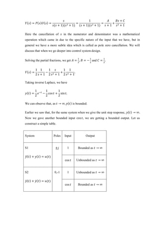
2. 𝑌( 𝑠) = 𝑃( 𝑠) 𝑈( 𝑠) =
1
𝑠2 + 1
𝑠
𝑠2 + 1
=
𝑠
(𝑠2 + 1)2
Now, we use a property of Laplace transform, the complex differentiation theorem.
𝐿[ 𝑡𝑓( 𝑡)] = −
𝑑𝐹(𝑠)
𝑑𝑠
Let us take 𝑓( 𝑡) = sin 𝑡,
𝐹( 𝑠) =
1
𝑠2 + 1
−
𝑑𝐹( 𝑠)
𝑑𝑠
=
2𝑠
( 𝑠2 + 1)2
,
𝑦( 𝑡) =
1
2
𝑡 sin 𝑡
We can observe that, as 𝑡 → ∞, 𝑦( 𝑡) → ∞.
(Refer Slide Time: 05:22)
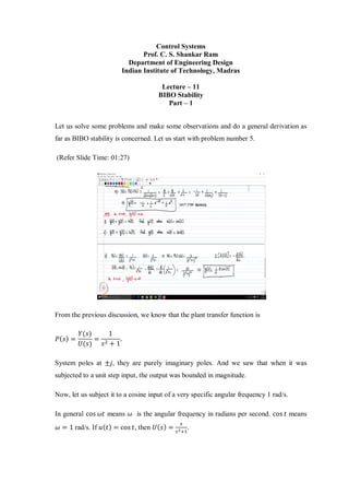
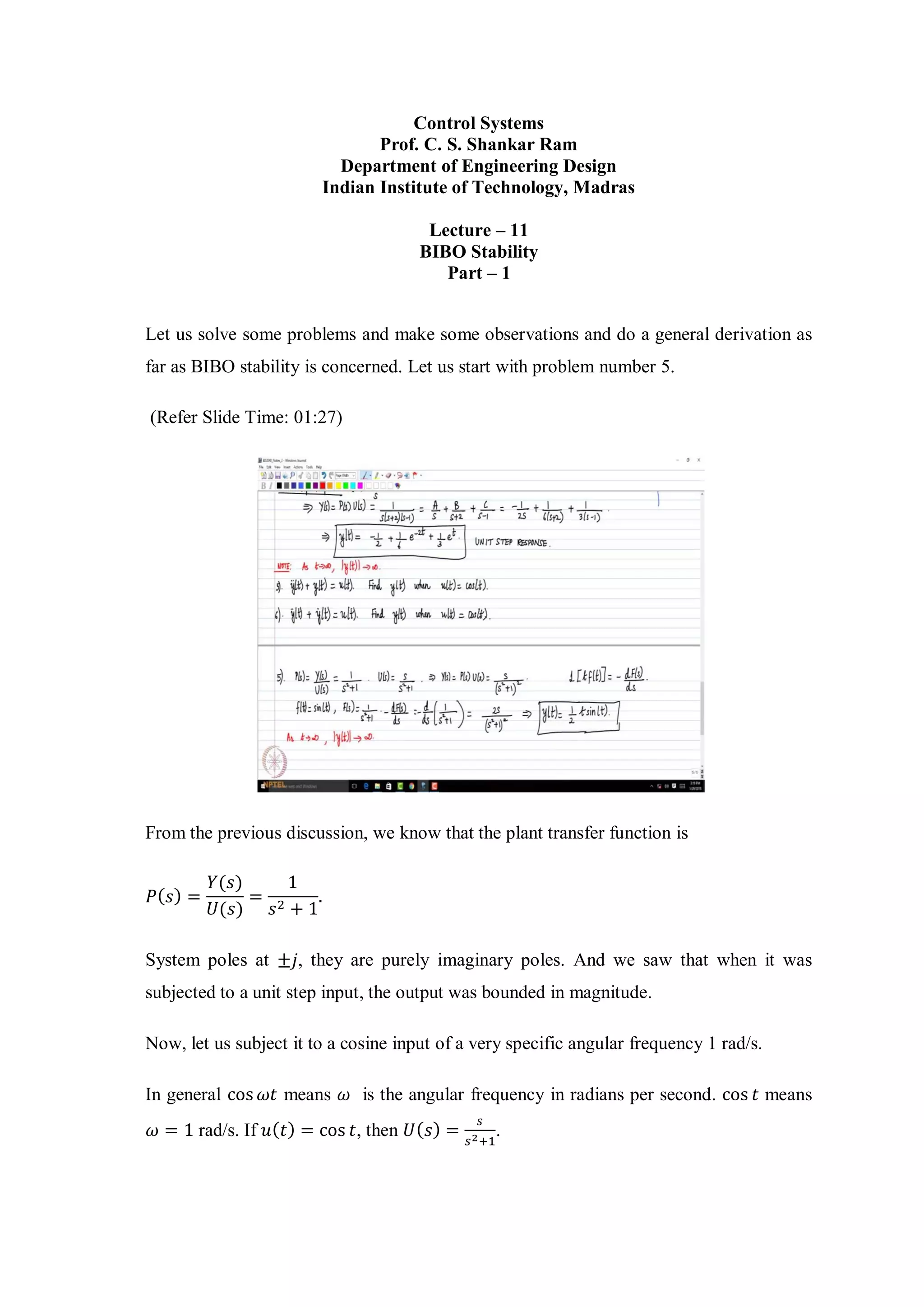
Now, let us solve problem number 6. We already know that the plant transfer function is
𝑃( 𝑠) =
𝑌(𝑠)
𝑈(𝑠)
=
1
𝑠2+𝑠
=
1
𝑠(𝑠+1)
.
𝑢( 𝑡) = cos 𝑡, then 𝑈( 𝑠) =
𝑠
𝑠2+1
.

3. 𝑌( 𝑠) = 𝑃( 𝑠) 𝑈( 𝑠) =
𝑠
𝑠(𝑠 + 1)(𝑠2 + 1)
=
1
(𝑠 + 1)(𝑠2 + 1)
=
𝐴
𝑠 + 1
+
𝐵𝑠 + 𝐶
𝑠2 + 1
Here the cancellation of 𝑠 in the numerator and denominator was a mathematical
operation which came in due to the specific nature of the input that we have, but in
general we have a more subtle idea which is called as pole zero cancellation. We will
discuss that when we go deeper into control system design.
Solving the partial fractions, we get 𝐴 =
1
2
, 𝐵 = −
1
2
and 𝐶 =
1
2
.
𝑌( 𝑠) =
1
2
1
𝑠 + 1
−
1
2
𝑠
𝑠2 + 1
+
1
2
1
𝑠2 + 1
.
Taking inverse Laplace, we have
𝑦( 𝑡) =
1
2
𝑒−𝑡
−
1
2
cos 𝑡 +
1
2
sin 𝑡.
We can observe that, as 𝑡 → ∞, 𝑦( 𝑡) is bounded.
Earlier we saw that, for the same system when we give the unit step response, 𝑦( 𝑡) → ∞.
Now we gave another bounded input cos 𝑡, we are getting a bounded output. Let us
construct a simple table.
System Poles Input Output
S1
𝑦̈( 𝑡) + 𝑦( 𝑡) = 𝑢(𝑡)
±𝑗 1 Bounded as 𝑡 → ∞
cos 𝑡 Unbounded as 𝑡 → ∞
S2
𝑦̈( 𝑡) + 𝑦̇( 𝑡) = 𝑢(𝑡)
0,-1 1 Unbounded as 𝑡 → ∞
cos 𝑡 Bounded as 𝑡 → ∞

4. It so turns out that if we use the definition of BIBO stability which states that a system is
BIBO stable if its output is bounded for all possible bounded inputs, we should brand
these two systems as unstable.
(Refer Slide Time: 14:14)
But, for the first system (S1) the output is unbounded, only if we give a sin 𝑡 or cos 𝑡 as
the input. For unit step input or any other bounded input like a sin or a cosine of any
angular frequency other than 1 rad/s, we can show that the output is going to be bounded.
It so turns out that only when the input becomes a sinusoid whose angular frequency is
equal to the magnitude of the poles on the imaginary axis, the output becomes
unbounded. For S1 the magnitude of poles on imaginary axis is 1. Some people will call
this class of systems as marginally stable or critically stable; that is the output is bounded
for all possible bounded inputs except one set. In strict parlance the system is unstable if
we use the definition as it is. We do not want to design such systems in practice. If we
encounter such systems we want to stabilize them.
If we have a mass spring damper system where there is no damper, we just have a mass
and the spring, the equation of motion will become 𝑀𝑥̈ + 𝑘𝑥 = 𝑓, the moment we give a
step input, the output will become unbounded.
Now, on the other hand if you look at system S2, it has a pole at the origin. If we have a
non-repeating pole at the origin you give a step input, the output is unbounded. But for
all other sinusoidal inputs, the output is bounded. That is the property of S2. We can see

5. that the output is unbounded only for one set of inputs. This result is true only if we have
for non repeating poles on the imaginary axis.
If you have a repeating pole on the imaginary axis. For example.
𝑃( 𝑠) =
1
𝑠2(𝑠 + 1)
(Refer Slide Time: 21:53)
The poles are at 0,0,-1, with the repeating poles this system is unstable.
Similarly, if you have another system where the transfer function is
𝑃( 𝑠) =
1
(𝑠2 + 1)2
The poles are +𝑗, +𝑗, −𝑗, −𝑗, this is unstable. The above concept of marginal stability or
critical stability applies, only if we have non repeating poles on the imaginary axis.
1. For BIBO stability, all poles of the plant transfer function must lie in the LHP or
in other words have negative real parts.
2. If there exists even one pole of the plant transfer function in the right half plane,
that is have has a positive real part, then the plant or the system is not BIBO
stable.

6. 3. If there are repeating poles of the plant transfer function on the imaginary axis (j
omega axis) with all remaining poles in the LHP, then system is not BIBO stable.
4. If there are non repeating poles of the plant transfer function on the imaginary
axis with all remaining poles in the LHP then the system is unstable or critically
stable.
Most textbook we will say it is critically or marginally stable, but if we strictly apply the
definition of BIBO stability it is unstable. If we are strict to that extent we should call
this as unstable, but if we can say the output is bounded only for one small group of
bounded inputs so we call it as critically stable or marginally stable.
That is basically some perspectives of how to interpret system stability when you have
poles, non-repeating poles on the imaginary axis, including the origin.
In condition number 1, if we have a system, we find the transfer function and figure out
that all poles of the system transfer function lie in the left half complex plane, is the
system BIBO stable? And answer is yes and we shall prove it later.