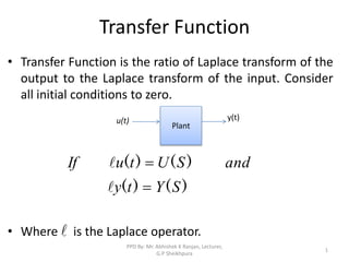
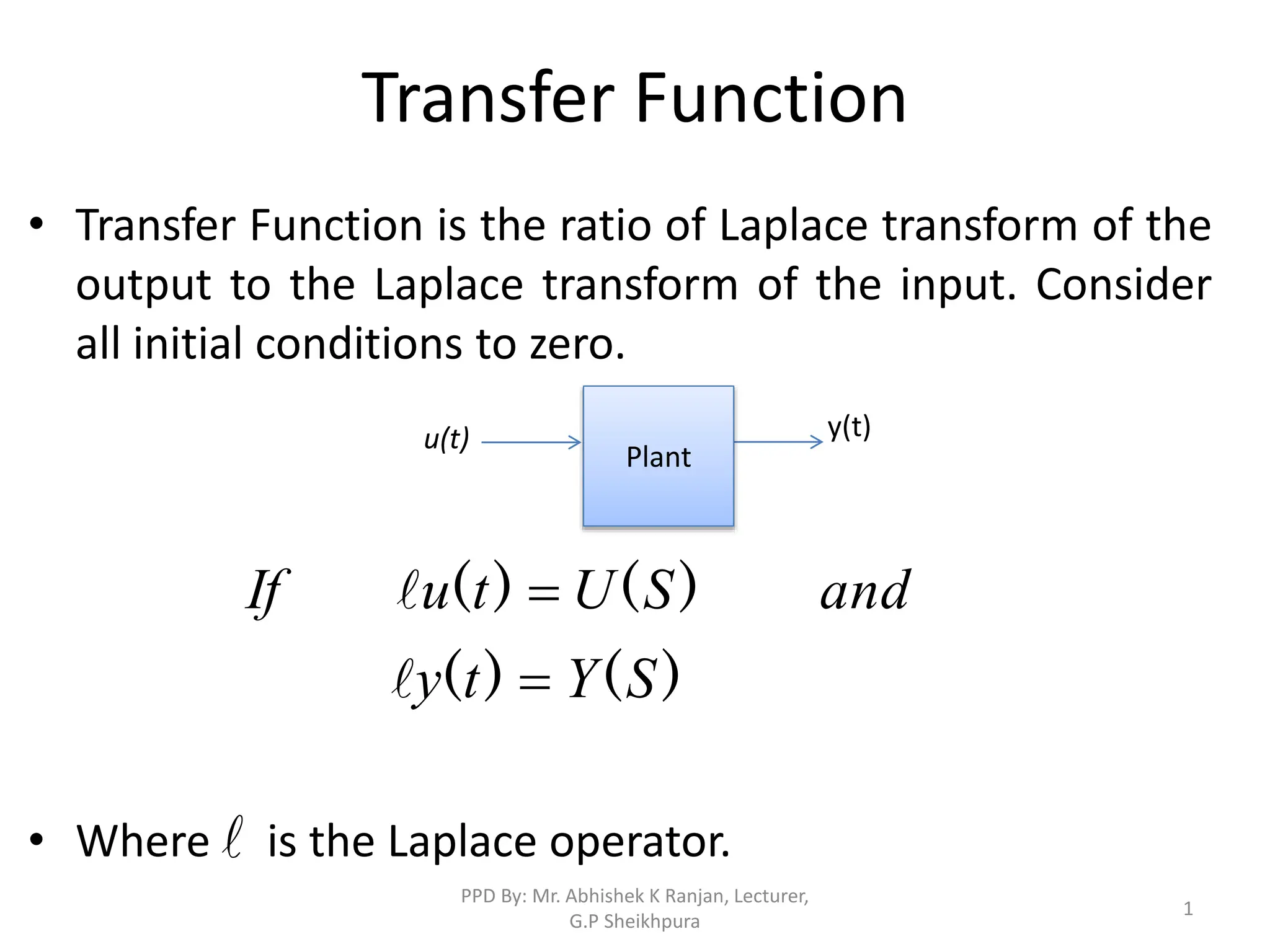
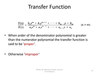
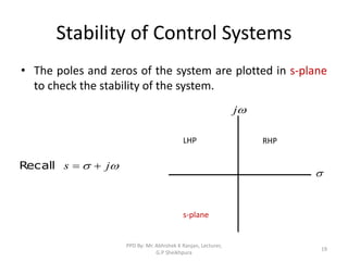
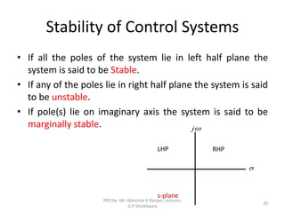
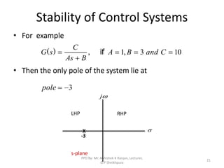
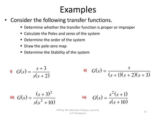
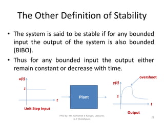
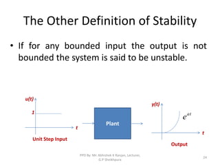
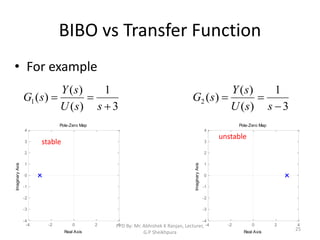
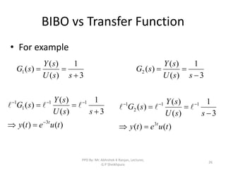
The document discusses transfer functions, which relate the Laplace transform of the output of a system to the Laplace transform of the input. It defines poles and zeros, and explains that stability is determined by whether the poles lie in the left or right half of the s-plane. It also discusses the BIBO definition of stability, where a system is stable if bounded inputs produce bounded outputs.

1. Transfer Function
• Transfer Function is the ratio of Laplace transform of the
output to the Laplace transform of the input. Consider
all initial conditions to zero.
• Where is the Laplace operator.
Plant
y(t)
u(t)
)
(
)
(
)
(
)
(
S
Y
t
y
and
S
U
t
u
If





1
PPD By: Mr. Abhishek K Ranjan, Lecturer,
G.P Sheikhpura

2. Transfer Function
• The transfer function G(S) of the plant is given as
G(S) Y(S)
U(S)
)
(
)
(
)
(
S
U
S
Y
S
G 
2
PPD By: Mr. Abhishek K Ranjan, Lecturer,
G.P Sheikhpura

3. Why Laplace Transform?
• Using Laplace transform, we can convert many common
functions into algebraic function of complex variable s.
• For example
• Where s is a complex variable (complex frequency) and
is given as
2
2





s
t
sin

a
s
e at


 1


 j
s 

3
PPD By: Mr. Abhishek K Ranjan, Lecturer,
G.P Sheikhpura

4. Laplace Transform of Derivatives
• Not only common function can be converted into
simple algebraic expressions but calculus operations
can also be converted into algebraic expressions.
• For example
)
0
(
)
(
)
(
x
s
sX
dt
t
dx



dt
dx
x
s
s
X
s
dt
t
x
d )
0
(
)
0
(
)
(
)
( 2
2
2





4
PPD By: Mr. Abhishek K Ranjan, Lecturer,
G.P Sheikhpura

5. Laplace Transform of Derivatives
• In general
• Where is the initial condition of the system.






n
k
k
k
n
n
n
n
x
s
s
X
s
dt
t
x
d
1
)
1
(
)
0
(
)
(
)
(

)
(0
x
5
PPD By: Mr. Abhishek K Ranjan, Lecturer,
G.P Sheikhpura

6. Laplace Transform of Integrals
)
(
1
)
( s
X
s
dt
t
x 


• The time domain integral becomes division by
s in frequency domain.
6
PPD By: Mr. Abhishek K Ranjan, Lecturer,
G.P Sheikhpura

7. Calculation of the Transfer Function
dt
t
dx
B
dt
t
dy
C
dt
t
x
d
A
)
(
)
(
)
(


2
2
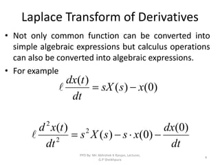
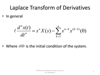
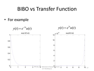
• Consider the following ODE where y(t) is input of the system and
x(t) is the output.
• or
• Taking the Laplace transform on either sides
)
(
'
)
(
'
)
(
'
' t
Bx
t
Cy
t
Ax 

)]
(
)
(
[
)]
(
)
(
[
)]
(
'
)
(
)
(
[ 0
0
0
0
2
x
s
sX
B
y
s
sY
C
x
sx
s
X
s
A 





7
PPD By: Mr. Abhishek K Ranjan, Lecturer,
G.P Sheikhpura

8. Calculation of the Transfer Function
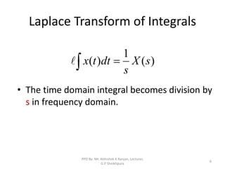
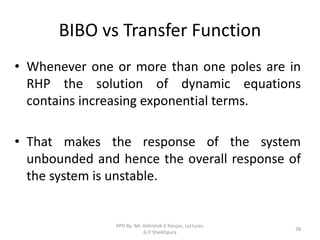
• Considering Initial conditions to zero in order to find the transfer
function of the system
• Rearranging the above equation
)]
(
)
(
[
)]
(
)
(
[
)]
(
'
)
(
)
(
[ 0
0
0
0
2
x
s
sX
B
y
s
sY
C
x
sx
s
X
s
A 





)
(
)
(
)
( s
BsX
s
CsY
s
X
As 

2
)
(
]
)[
(
)
(
)
(
)
(
s
CsY
Bs
As
s
X
s
CsY
s
BsX
s
X
As




2
2
B
As
C
Bs
As
Cs
s
Y
s
X



 2
)
(
)
(
8
PPD By: Mr. Abhishek K Ranjan, Lecturer,
G.P Sheikhpura

9. Transfer Function
• In general
• Where x is the input of the system and y is the output of
the system.
9
PPD By: Mr. Abhishek K Ranjan, Lecturer,
G.P Sheikhpura

10. Transfer Function
• When order of the denominator polynomial is greater
than the numerator polynomial the transfer function is
said to be ‘proper’.
• Otherwise ‘improper’
10
PPD By: Mr. Abhishek K Ranjan, Lecturer,
G.P Sheikhpura

11. Transfer Function
• Transfer function can be used to check
– The stability of the system
– Time domain and frequency domain characteristics of the
system
– Response of the system for any given input
11
PPD By: Mr. Abhishek K Ranjan, Lecturer,
G.P Sheikhpura

12. Stability of Control System
• There are several meanings of stability, in general
there are two kinds of stability definitions in control
system study.
– Absolute Stability
– Relative Stability
12
PPD By: Mr. Abhishek K Ranjan, Lecturer,
G.P Sheikhpura

13. Stability of Control System
• Roots of denominator polynomial of a transfer
function are called ‘poles’.
• The roots of numerator polynomials of a
transfer function are called ‘zeros’.
13
PPD By: Mr. Abhishek K Ranjan, Lecturer,
G.P Sheikhpura

14. Stability of Control System
• Poles of the system are represented by ‘x’ and
zeros of the system are represented by ‘o’.
• System order is always equal to number of
poles of the transfer function.
• Following transfer function represents nth
order plant (i.e., any physical object).
14
PPD By: Mr. Abhishek K Ranjan, Lecturer,
G.P Sheikhpura

15. Stability of Control System
• Poles is also defined as “it is the frequency at which
system becomes infinite”. Hence the name pole
where field is infinite.
• Zero is the frequency at which system becomes 0.
15
PPD By: Mr. Abhishek K Ranjan, Lecturer,
G.P Sheikhpura

16. Stability of Control System
• Poles is also defined as “it is the frequency at which
system becomes infinite”.
• Like a magnetic pole or black hole.
16

17. Example
• Consider the Transfer function calculated in previous
slides.
• The only pole of the system is
17
B
As
C
s
Y
s
X
s
G



)
(
)
(
)
(
0

 B
As
is
polynomial
r
denominato
the
A
B
s 

PPD By: Mr. Abhishek K Ranjan, Lecturer,
G.P Sheikhpura

18. Examples
• Consider the following transfer functions.
– Determine
• Whether the transfer function is proper or improper
• Poles of the system
• zeros of the system
• Order of the system
18
)
(
)
(
2
3



s
s
s
s
G
)
)(
)(
(
)
(
3
2
1 



s
s
s
s
s
G
)
(
)
(
)
(
10
3
2
2



s
s
s
s
G
)
(
)
(
)
(
10
1
2



s
s
s
s
s
G
i) ii)
iii) iv)
PPD By: Mr. Abhishek K Ranjan, Lecturer,
G.P Sheikhpura

19. Stability of Control Systems
• The poles and zeros of the system are plotted in s-plane
to check the stability of the system.
19
s-plane
LHP RHP


j

 j
s 

Recall
PPD By: Mr. Abhishek K Ranjan, Lecturer,
G.P Sheikhpura

20. Stability of Control Systems
• If all the poles of the system lie in left half plane the
system is said to be Stable.
• If any of the poles lie in right half plane the system is said
to be unstable.
• If pole(s) lie on imaginary axis the system is said to be
marginally stable.
20
s-plane
LHP RHP


j
PPD By: Mr. Abhishek K Ranjan, Lecturer,
G.P Sheikhpura

21. Stability of Control Systems
• For example
• Then the only pole of the system lie at
21
10
3
1 



 C
and
B
A
B
As
C
s
G if ,
,
)
(
3


pole
s-plane
LHP RHP


j
X
-3
PPD By: Mr. Abhishek K Ranjan, Lecturer,
G.P Sheikhpura

22. Examples
• Consider the following transfer functions.
 Determine whether the transfer function is proper or improper
 Calculate the Poles and zeros of the system
 Determine the order of the system
 Draw the pole-zero map
 Determine the Stability of the system
22
)
(
)
(
2
3



s
s
s
s
G
)
)(
)(
(
)
(
3
2
1 



s
s
s
s
s
G
)
(
)
(
)
(
10
3
2
2



s
s
s
s
G
)
(
)
(
)
(
10
1
2



s
s
s
s
s
G
i) ii)
iii) iv)
PPD By: Mr. Abhishek K Ranjan, Lecturer,
G.P Sheikhpura

23. The Other Definition of Stability
• The system is said to be stable if for any bounded
input the output of the system is also bounded
(BIBO).
• Thus for any bounded input the output either
remain constant or decrease with time.
23
u(t)
t
1
Unit Step Input
Plant
y(t)
t
Output
1
overshoot
PPD By: Mr. Abhishek K Ranjan, Lecturer,
G.P Sheikhpura

24. The Other Definition of Stability
• If for any bounded input the output is not
bounded the system is said to be unstable.
24
u(t)
t
1
Unit Step Input
Plant
y(t)
t
Output
at
e
PPD By: Mr. Abhishek K Ranjan, Lecturer,
G.P Sheikhpura

25. BIBO vs Transfer Function
• For example
3
1
)
(
)
(
)
(
1



s
s
U
s
Y
s
G
3
1
)
(
)
(
)
(
2



s
s
U
s
Y
s
G
-4 -2 0 2 4
-4
-3
-2
-1
0
1
2
3
4
Pole-Zero Map
Real Axis
Imaginary
Axis
-4 -2 0 2 4
-4
-3
-2
-1
0
1
2
3
4
Pole-Zero Map
Real Axis
Imaginary
Axis
stable
unstable
PPD By: Mr. Abhishek K Ranjan, Lecturer,
G.P Sheikhpura
25

26. BIBO vs Transfer Function
• For example
3
1
)
(
)
(
)
(
1



s
s
U
s
Y
s
G
3
1
)
(
)
(
)
(
2



s
s
U
s
Y
s
G
)
(
)
(
3
1
)
(
)
(
)
(
3
1
1
1
1
t
u
e
t
y
s
s
U
s
Y
s
G
t








 


)
(
)
(
3
1
)
(
)
(
)
(
3
1
1
2
1
t
u
e
t
y
s
s
U
s
Y
s
G
t




 





PPD By: Mr. Abhishek K Ranjan, Lecturer,
G.P Sheikhpura
26

27. BIBO vs Transfer Function
• For example
)
(
)
( 3
t
u
e
t
y t

 )
(
)
( 3
t
u
e
t
y t

0 1 2 3 4
0
0.2
0.4
0.6
0.8
1
exp(-3t)*u(t)
0 2 4 6 8 10
0
2
4
6
8
10
12
x 10
12
exp(3t)*u(t)
PPD By: Mr. Abhishek K Ranjan, Lecturer,
G.P Sheikhpura
27

28. BIBO vs Transfer Function
• Whenever one or more than one poles are in
RHP the solution of dynamic equations
contains increasing exponential terms.
• That makes the response of the system
unbounded and hence the overall response of
the system is unstable.
PPD By: Mr. Abhishek K Ranjan, Lecturer,
G.P Sheikhpura
28

29. Summary
• Transfer Function
• The Order of Control Systems
• Poles, Zeros
• Stability
• BIBO
29
PPD By: Mr. Abhishek K Ranjan, Lecturer,
G.P Sheikhpura