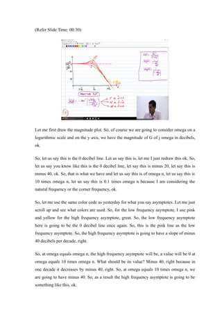
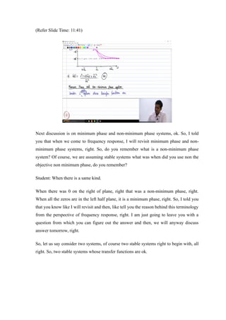
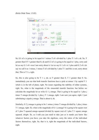
Control Systems
Prof. C. S. Shankar Ram
Department of Engineering Design
Indian Institute of Technology, Madras
Lecture - 54
Bode Plot 3
Part - 2
(Refer Slide Time: 00:15)
So, now let me go and draw the bode plot, with all this background. Let us go and now, I
construct bode diagram for this particular second order transfer function, ok.
So, how do we, how does it look? So, let us draw the bode plot.
(Refer Slide Time: 00:30)
Let me first draw the magnitude plot. So, of course we are going to consider omega on a
logarithmic scale and on the y axis, we have the magnitude of G of j omega in decibels,
ok.
So, let us say this is the 0 decibel line. Let us say this is, let me I just redraw this ok. So,
let us say you know like this is the 0 decibel line, let say this is minus 20, let say this is
minus 40, ok. So, that is what we have and let us say this is of omega n, let us say this is
10 times omega n, let us say this is 0.1 times omega n because I am considering the
natural frequency or the corner frequency, ok.
So, let me use the same color code as yesterday for what you say asymptotes. Let me just
scroll up and see what colors are used. So, for the low frequency asymptote, I use pink
and yellow for the high frequency asymptote, great. So, the low frequency asymptote
here is going to be the 0 decibel line once again. So, this is the pink line as the low
frequency asymptote. So, the high frequency asymptote is going to have a slope of minus
40 decibels per decade, right.
So, at omega equals omega n, the high frequency asymptote will be, a value will be 0 at
omega equals 10 times omega n. What should be its value? Minus 40, right because in
one decade it decreases by minus 40, right. So, at omega equals 10 times omega n, we
are going to have minus 40. So, as a result the high frequency asymptote is going to be
something like this, ok.
So, I am just extending it to show it graphically ok, but this is a high frequency
asymptote. The slope is minus 40 decibels per decade, ok. Now, the point is the actual
curve depends on the value of zeta, ok. So, please note that the maximum amplitude
occurs at omega equals omega n times square root of 1 minus 2 zeta squared, ok. That is
the resonant frequency. So, as zeta increases from 0, what do you think will happen to
this resonant frequency? Will it become less than? Will it become red? Go towards the
left of omega and further to the left? Yes because as zeta increases, you see that 1 minus
zeta 2 zeta square decreases.
So, as a result as zeta increases from 0, the further the increase in zeta, the further is the
shift of the resonant frequency to the left from the natural frequency. So, I am just going
to draw a family of curves which will essentially tell us how the natural frequency curve
looks like, ok. So, this is the actual curve. So, let us say you know at low damping ratios
I have this. Ultimately it will go and contain as the damping ratio increases, the peak
essentially shifts further and further to the left, but anyway after some time everything
goes to the high frequency asymptote, right.
So, I am just drawing a freehand sketch. So, please pardon the approximate diagram, ok.
So, what happens is that this is how the peak changes, right as zeta increases. Of course,
after zeta greater than 1 by root 2, you see that the maximum value never crosses zero
decibels, ok. That means, that there is no peak assets for zeta greater than 1 by root 2.
So, that is why the maximum value is 0 decibels, right. So, that is it. The low frequency
asymptote is the highest value, ok. So, that is what happens. Of course, what happens to
this magnitude plot for an undamped system, what do you think will happen? You will
see that once again low frequency asymptote will be 0 decibels, high frequency
asymptote will have a slope of minus 40 decibels per decade, but what will happen at
omega equals omega n you will see that the amplitude will blow up to infinity, right.
So, essentially that is what we have, right. So, essentially it is going to be a very high
amplitude. So, what do I mean by that. Let us say you know like let us say we consider
the undamped system omega n squared divided by s square plus omega n squared. What
is going to be G of j omega? It is going to be 1 divided by 1 minus omega squared by
omega n square, right. So, what is the amplitude? It is the same, right; so essentially, but
anyway there is no imaginary term, ok. So, you get the same thing in a sense, right.
So, if I rewrite this, this is going to be 1 minus omega square by omega n square, right.
Of course, the absolute value, right. So, you need to take the, so you can immediately see
that what happens as omega tends to omega n. The amplitude just blows off to infinity,
right. So, that is what you have when you have what to say for an undamped system, ok.
So, this is just an asset, right ok. Now, this is the magnitude plot, ok. So, this is the
magnitude plot of the second order term that we have been considering.
Now, what about the phase? So, please note that the phase is going to be G of j of phase
of G of j omega was essentially what minus tan inverse of 2 zeta omega by omega n
divided by 1 minus omega squared by omega n square. So, one can immediately figure
out that this phase goes to 0 degrees as omega tends to 0. This goes to minus 90 degrees
as omega equals omega n, ok. This essentially goes to minus 180 degrees as omega tends
to infinity, ok.
So, this is what happens to this to the phase plot of this particular factor. So, if you want
to plot the phase plot; what will happen as a following?
(Refer Slide Time: 08:25)
So, let me plot the phase plot of this particular transfer function. So, this we are going to
plot in degrees. So, let us say this is 0 or minus 90, then minus 180, then we have omega
n 10 times omega n and 0.1 times omega n, ok.
So, what is going to happen is the following. So, 0 to 1 minus 180 are the two bounds
and at omega equals omega n, you are going to have minus 90, right. So, what will
happen to the phase plot is following. So, as zeta starts to increase from 0, we are going
to have the phase plot, go something like this and as zeta keeps on increasing, it becomes
like this, ok. We are going to get a family of course, right.
So, depending on the value of zeta, so this is for a lower zeta, ok. So, you are going to
get a stronger in function, ok. So, this is what happens as zeta increase, ok. So, that is
just a family. Of course, you know just to show you how the phase changes for this
particular factor, as zeta increases from 0, ok. So, that is the phase of this particular
second order transfer function and if you consider the reciprocal of that which is s square
takes 2 zeta omega n s plus omega n squared divided by omega n square. So, what will
happen? You will just get the mirror image, right about the 0 decibel line, but I leave that
to as a homework, ok. So, the seventh factor is essentially this which is essentially the
reciprocal of the factor that we just consider. So, what I want you to do is, then do it as
homework, ok.
So, it just will be a mirror image of this one, right. Any questions here; fine. So, I am just
going to leave you with one more question to think about right and then, like we will
continue and discuss it in the next class, right and then, we will do an example, ok. The
next class we are going to do an example of the construction of the bode diagram, but I
am just going to leave you with a question to essentially think about. So, we are done
with this, ok.
(Refer Slide Time: 11:41)
Next discussion is on minimum phase and non-minimum phase systems, ok. So, I told
you that when we come to frequency response, I will revisit minimum phase and non-
minimum phase systems, right. So, do you remember what is a non-minimum phase
system? Of course, we are assuming stable systems what was when did you use non the
objective non minimum phase, do you remember?
Student: When there is a same kind.
When there was 0 on the right of plane, right that was a non-minimum phase, right.
When all the zeros are in the left half plane, it is a minimum phase, right. So, I told you
that you know like I will revisit and then, like tell you the reason behind this terminology
from the perspective of frequency response, right. I am just going to leave you with a
question from which you can figure out the answer and then, we will anyway discuss
answer tomorrow, right.
So, let us say consider two systems, of course two stable systems right to begin with, all
right. So, two stable systems whose transfer functions are ok.
(Refer Slide Time: 13:02)
So, G1 of s is going to be equal to 1 minus T of s divided by 1 plus T 1 of s, ok. So, T
greater than 0 T 1 greater than 0, ok and G 2 of s is going to be equal to 1 plus, sorry and
let us say G 1 of s was I am sorry about it. Let us say G 1 of s is 1 plus and G 2 of s let
say we call it as 1 minus, 1 minus T of s divided by 1 plus T 1 and this is not, sorry about
that. This is T 1 s, right.
So, this is also going to be T 1 s, ok; so T greater than 0, T 1 greater than 0. So,
immediately you see that both transfer functions have a pole at minus 1 by capital T 1
which is in the left of plane, right. No issues regarding the stability of either systems,
right. So, what is the magnitude of the sinusoidal transfer function, but before we
calculate the magnitude let us write G 1 j omega. That is going to be equal to 1 plus j
times T omega divided by 1 plus j T 1 omega, right. I am sure you agree, right. I just
substituting s equals j omega. That is about it, ok.
Similarly, G 2 j omega is going to be 1 minus j times T omega divided by 1 plus j times
T 1 omega, right. So, what is the magnitude of G 1 j omega? It is going to be square root
of 1 plus T squared omega squared divided by square root of 1 plus T 1 square omega
squared, alright. So, as I told you just need to take just as it stands you know like
whatever factors you have, you take the algebraic, sorry the ratios of the individual
factors themselves, right. So, that is it, right the magnitude of the individual factors,
right.
So, now what is the magnitude of G 2 j omega? It is going to be 1 square root of 1 plus T
squared omega squared that would be square root of 1 plus T 1 square omega square. So,
what can you say about the two magnitudes same, right. They are equal in magnitude,
right for all omega.
So, you give me any omega, you can see that the magnitude of G 1 j omega and
magnitude of G 2 j omega are the same. Now, let us look at magnet, a phase of G 1 j
omega, ok. What is the phase of G 1 j omega? It is going to be tan inverse of T omega
minus tan inverse of T 1 omega, right. So, then what is the phase of G 2 j omega? It is
going to be minus tan inverse of T omega minus tan inverse of T 1, right.
So, what do you think happens to the phase of G 1 j omega? As omega tends to infinity
tends to 0, right. What can you say about the phase of G 2 j omega. As omega tends to
infinity, it tends to minus 180 which has the minimum phase G 1, right and see G 2 j
omega phase tends to minus 180, G 1 tends to 0, right. So, I hope it is clear.
Now, why the system with the transfer function G 1 is called minimum phase and why
the system is the transfer function G 2 j G 2 s is called non-minimum phase? So, in
essence what we are saying is that if you give me two systems whose transfer functions
have the same magnitude characteristics, the minimum phase system will have the lower
phase. Of course, the thing is that like we are only looking at the magnitude per, right
with this, with the essentially sin, right.
So, essentially it will have the minimal phase like of the two, ok. That is why it is called
as a minimum phase system. The question I am going to leave you with is that how can
we generalize it for any nth order system? Let us say you know like what was our
general transfer function, you remember G of s was n of s by d of s, right. N of s was a
polynomial of order m d of s was a polynomial of order n, right.
How can you generalize it for any nth order system? So, that is a question I leave you
with or if I give you bode plot of a transfer function by looking at it, can you get the
relative degree of the system. What I mean by the relative degree is n. What is called as n
minus m? N minus m is the relative degree of the transfer function and also, figure out
whether its minimum phase or non-minimum phase, ok. Can we do that?
So, those are questions I am going to leave you with, I am going to come and discuss the
answers tomorrow, but please think about them, ok. We will discuss those answers
tomorrow and then, we will also do an example problem, right and tomorrow's class for
the bode diagram which would complete our discussion on bode plots fine, ok. So, I will
stop here. I will see you in the next class.
Thank you.

Lec54

  • 1.
    Control Systems Prof. C.S. Shankar Ram Department of Engineering Design Indian Institute of Technology, Madras Lecture - 54 Bode Plot 3 Part - 2 (Refer Slide Time: 00:15) So, now let me go and draw the bode plot, with all this background. Let us go and now, I construct bode diagram for this particular second order transfer function, ok. So, how do we, how does it look? So, let us draw the bode plot.
  • 2.
    (Refer Slide Time:00:30) Let me first draw the magnitude plot. So, of course we are going to consider omega on a logarithmic scale and on the y axis, we have the magnitude of G of j omega in decibels, ok. So, let us say this is the 0 decibel line. Let us say this is, let me I just redraw this ok. So, let us say you know like this is the 0 decibel line, let say this is minus 20, let say this is minus 40, ok. So, that is what we have and let us say this is of omega n, let us say this is 10 times omega n, let us say this is 0.1 times omega n because I am considering the natural frequency or the corner frequency, ok. So, let me use the same color code as yesterday for what you say asymptotes. Let me just scroll up and see what colors are used. So, for the low frequency asymptote, I use pink and yellow for the high frequency asymptote, great. So, the low frequency asymptote here is going to be the 0 decibel line once again. So, this is the pink line as the low frequency asymptote. So, the high frequency asymptote is going to have a slope of minus 40 decibels per decade, right. So, at omega equals omega n, the high frequency asymptote will be, a value will be 0 at omega equals 10 times omega n. What should be its value? Minus 40, right because in one decade it decreases by minus 40, right. So, at omega equals 10 times omega n, we are going to have minus 40. So, as a result the high frequency asymptote is going to be something like this, ok.
  • 3.
    So, I amjust extending it to show it graphically ok, but this is a high frequency asymptote. The slope is minus 40 decibels per decade, ok. Now, the point is the actual curve depends on the value of zeta, ok. So, please note that the maximum amplitude occurs at omega equals omega n times square root of 1 minus 2 zeta squared, ok. That is the resonant frequency. So, as zeta increases from 0, what do you think will happen to this resonant frequency? Will it become less than? Will it become red? Go towards the left of omega and further to the left? Yes because as zeta increases, you see that 1 minus zeta 2 zeta square decreases. So, as a result as zeta increases from 0, the further the increase in zeta, the further is the shift of the resonant frequency to the left from the natural frequency. So, I am just going to draw a family of curves which will essentially tell us how the natural frequency curve looks like, ok. So, this is the actual curve. So, let us say you know at low damping ratios I have this. Ultimately it will go and contain as the damping ratio increases, the peak essentially shifts further and further to the left, but anyway after some time everything goes to the high frequency asymptote, right. So, I am just drawing a freehand sketch. So, please pardon the approximate diagram, ok. So, what happens is that this is how the peak changes, right as zeta increases. Of course, after zeta greater than 1 by root 2, you see that the maximum value never crosses zero decibels, ok. That means, that there is no peak assets for zeta greater than 1 by root 2. So, that is why the maximum value is 0 decibels, right. So, that is it. The low frequency asymptote is the highest value, ok. So, that is what happens. Of course, what happens to this magnitude plot for an undamped system, what do you think will happen? You will see that once again low frequency asymptote will be 0 decibels, high frequency asymptote will have a slope of minus 40 decibels per decade, but what will happen at omega equals omega n you will see that the amplitude will blow up to infinity, right. So, essentially that is what we have, right. So, essentially it is going to be a very high amplitude. So, what do I mean by that. Let us say you know like let us say we consider the undamped system omega n squared divided by s square plus omega n squared. What is going to be G of j omega? It is going to be 1 divided by 1 minus omega squared by omega n square, right. So, what is the amplitude? It is the same, right; so essentially, but anyway there is no imaginary term, ok. So, you get the same thing in a sense, right.
  • 4.
    So, if Irewrite this, this is going to be 1 minus omega square by omega n square, right. Of course, the absolute value, right. So, you need to take the, so you can immediately see that what happens as omega tends to omega n. The amplitude just blows off to infinity, right. So, that is what you have when you have what to say for an undamped system, ok. So, this is just an asset, right ok. Now, this is the magnitude plot, ok. So, this is the magnitude plot of the second order term that we have been considering. Now, what about the phase? So, please note that the phase is going to be G of j of phase of G of j omega was essentially what minus tan inverse of 2 zeta omega by omega n divided by 1 minus omega squared by omega n square. So, one can immediately figure out that this phase goes to 0 degrees as omega tends to 0. This goes to minus 90 degrees as omega equals omega n, ok. This essentially goes to minus 180 degrees as omega tends to infinity, ok. So, this is what happens to this to the phase plot of this particular factor. So, if you want to plot the phase plot; what will happen as a following? (Refer Slide Time: 08:25) So, let me plot the phase plot of this particular transfer function. So, this we are going to plot in degrees. So, let us say this is 0 or minus 90, then minus 180, then we have omega n 10 times omega n and 0.1 times omega n, ok.
  • 5.
    So, what isgoing to happen is the following. So, 0 to 1 minus 180 are the two bounds and at omega equals omega n, you are going to have minus 90, right. So, what will happen to the phase plot is following. So, as zeta starts to increase from 0, we are going to have the phase plot, go something like this and as zeta keeps on increasing, it becomes like this, ok. We are going to get a family of course, right. So, depending on the value of zeta, so this is for a lower zeta, ok. So, you are going to get a stronger in function, ok. So, this is what happens as zeta increase, ok. So, that is just a family. Of course, you know just to show you how the phase changes for this particular factor, as zeta increases from 0, ok. So, that is the phase of this particular second order transfer function and if you consider the reciprocal of that which is s square takes 2 zeta omega n s plus omega n squared divided by omega n square. So, what will happen? You will just get the mirror image, right about the 0 decibel line, but I leave that to as a homework, ok. So, the seventh factor is essentially this which is essentially the reciprocal of the factor that we just consider. So, what I want you to do is, then do it as homework, ok. So, it just will be a mirror image of this one, right. Any questions here; fine. So, I am just going to leave you with one more question to think about right and then, like we will continue and discuss it in the next class, right and then, we will do an example, ok. The next class we are going to do an example of the construction of the bode diagram, but I am just going to leave you with a question to essentially think about. So, we are done with this, ok.
  • 6.
    (Refer Slide Time:11:41) Next discussion is on minimum phase and non-minimum phase systems, ok. So, I told you that when we come to frequency response, I will revisit minimum phase and non- minimum phase systems, right. So, do you remember what is a non-minimum phase system? Of course, we are assuming stable systems what was when did you use non the objective non minimum phase, do you remember? Student: When there is a same kind. When there was 0 on the right of plane, right that was a non-minimum phase, right. When all the zeros are in the left half plane, it is a minimum phase, right. So, I told you that you know like I will revisit and then, like tell you the reason behind this terminology from the perspective of frequency response, right. I am just going to leave you with a question from which you can figure out the answer and then, we will anyway discuss answer tomorrow, right. So, let us say consider two systems, of course two stable systems right to begin with, all right. So, two stable systems whose transfer functions are ok.
  • 7.
    (Refer Slide Time:13:02) So, G1 of s is going to be equal to 1 minus T of s divided by 1 plus T 1 of s, ok. So, T greater than 0 T 1 greater than 0, ok and G 2 of s is going to be equal to 1 plus, sorry and let us say G 1 of s was I am sorry about it. Let us say G 1 of s is 1 plus and G 2 of s let say we call it as 1 minus, 1 minus T of s divided by 1 plus T 1 and this is not, sorry about that. This is T 1 s, right. So, this is also going to be T 1 s, ok; so T greater than 0, T 1 greater than 0. So, immediately you see that both transfer functions have a pole at minus 1 by capital T 1 which is in the left of plane, right. No issues regarding the stability of either systems, right. So, what is the magnitude of the sinusoidal transfer function, but before we calculate the magnitude let us write G 1 j omega. That is going to be equal to 1 plus j times T omega divided by 1 plus j T 1 omega, right. I am sure you agree, right. I just substituting s equals j omega. That is about it, ok. Similarly, G 2 j omega is going to be 1 minus j times T omega divided by 1 plus j times T 1 omega, right. So, what is the magnitude of G 1 j omega? It is going to be square root of 1 plus T squared omega squared divided by square root of 1 plus T 1 square omega squared, alright. So, as I told you just need to take just as it stands you know like whatever factors you have, you take the algebraic, sorry the ratios of the individual factors themselves, right. So, that is it, right the magnitude of the individual factors, right.
  • 8.
    So, now whatis the magnitude of G 2 j omega? It is going to be 1 square root of 1 plus T squared omega squared that would be square root of 1 plus T 1 square omega square. So, what can you say about the two magnitudes same, right. They are equal in magnitude, right for all omega. So, you give me any omega, you can see that the magnitude of G 1 j omega and magnitude of G 2 j omega are the same. Now, let us look at magnet, a phase of G 1 j omega, ok. What is the phase of G 1 j omega? It is going to be tan inverse of T omega minus tan inverse of T 1 omega, right. So, then what is the phase of G 2 j omega? It is going to be minus tan inverse of T omega minus tan inverse of T 1, right. So, what do you think happens to the phase of G 1 j omega? As omega tends to infinity tends to 0, right. What can you say about the phase of G 2 j omega. As omega tends to infinity, it tends to minus 180 which has the minimum phase G 1, right and see G 2 j omega phase tends to minus 180, G 1 tends to 0, right. So, I hope it is clear. Now, why the system with the transfer function G 1 is called minimum phase and why the system is the transfer function G 2 j G 2 s is called non-minimum phase? So, in essence what we are saying is that if you give me two systems whose transfer functions have the same magnitude characteristics, the minimum phase system will have the lower phase. Of course, the thing is that like we are only looking at the magnitude per, right with this, with the essentially sin, right. So, essentially it will have the minimal phase like of the two, ok. That is why it is called as a minimum phase system. The question I am going to leave you with is that how can we generalize it for any nth order system? Let us say you know like what was our general transfer function, you remember G of s was n of s by d of s, right. N of s was a polynomial of order m d of s was a polynomial of order n, right. How can you generalize it for any nth order system? So, that is a question I leave you with or if I give you bode plot of a transfer function by looking at it, can you get the relative degree of the system. What I mean by the relative degree is n. What is called as n minus m? N minus m is the relative degree of the transfer function and also, figure out whether its minimum phase or non-minimum phase, ok. Can we do that?
  • 9.
    So, those arequestions I am going to leave you with, I am going to come and discuss the answers tomorrow, but please think about them, ok. We will discuss those answers tomorrow and then, we will also do an example problem, right and tomorrow's class for the bode diagram which would complete our discussion on bode plots fine, ok. So, I will stop here. I will see you in the next class. Thank you.