
Recommended
More Related Content
What's hot
What's hot (19)
Viewers also liked
Viewers also liked (20)
Similar to Ldo project
Similar to Ldo project (20)
Ldo project
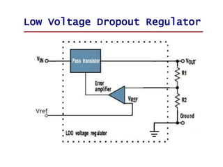
- 1. Low Voltage Dropout Regulator
- 2. Goal: Design a voltage regulator to provide an output voltage of 3.3V
- 3. For the calculations we assume the following constants: - Pass transistor current = 1ma - Vout = 3.3V - Dropout voltage = - VDD=5V -
- 4. Calculations: - Calculation of a range of Vbias1 1. To find Ibias1: From the desired a photodiode range, the minimum value of Ibias1: VGS3 =Vphmin Ibias1 = ½ K1(W/L)3 (VGS3 -VTHN )2 = ½ * 50 * 10-6 A/V2 * 3µm/0.6µm * (0.8V – 0.617)2 = 4.186µA =4µA The maximum value of Ibias1: Ibias1 = ½ K1(W/L)3 (VGS3 -VTHN )2 = ½ * 50 * 10-6 A/V2 * 3µm/0.6µm * (3.0V – 0.617)2 = 0.7mA
- 5. Calculations: - Calculation of a range of Vbias1 2. To find Vbias1: Next we find the value of Vbias1 given by Vbias1 = VDD – VGS0 = VDD - √[(2Ibias1)/(K2 (W/L)0 ] – VTHp Vbias1 = VDD – VGS0 = VDD - √[ (2Ibias1)/(K2 (W/L)0 ] – VTHp p The maximum value of Vbias1: Vbias1(max) = 5V - √[(2*4µA)/(19.1µA/V2* 20µm/0.6µm)] – 0.915V =1.026 = 4V The minimum value of Vbias1: Vbias1(min) = VDD – VGS0 = 5V- √[(2*0.7*10-3 )/25* 10-6 /V2 * 20µm/0.6µm) – 0.915V = 2.8V
- 6. Calculations: - Calculation of sizes of the transistors M5, M4 1. To determine W5 From requirement to keep M5 in saturation region: VTH ≤VGS5 = Vbias1(min) + VTHp – Vph (max) = 2.8V +0.9V – 3.0V = 0.7V W5 = (2InL5 )/(K1 (VGS5 -VTHN )2 ) = (2 * 1.2µA * 0.6µm)/(50µA/V2 * (0.7V – 0.617V)2 ) = 4µm
- 7. Calculations: - Calculation of sizes of the transistors M5, M4 2. To determine W4 VDS4 ≥VGS4 – VTHN VDS4 = Vph (min) = 0.8V Assumed VGS4 = 0.75V W4 = (2InL4 )/(K1 (VGS4 -VTHN )2 ) = (2 * 1.2µA * 0.6µm)/(50µA/V2 * (0.75V – 0.617V)2 ) = 1.60µm
- 8. Calculations: - Calculation of the gain for the current mirror transistors M1, M2, M7 1. To find VGS for M1, M2, M7 VGS1 = VDS1 = VGS2 = VGS1 = √[(2Iout)/(K2 (W/L)2,7 ] + VTHp = √(2 * 1.2µA)/(25µA/V2 * (20/2.4)) + 0.915V = 0.107V + 0.915V = 1V
- 9. Calculations: - Calculation of the gain for the current mirror transistors M1, M2, M7 2. To find VDS for current mirror: Next we find VDS2 and VDS7 (which are the same in value) VDS2,7 = VDD – VDS6 = VDD - √[(2Iout)/(K1 (W/L)6 ] - VTHN = 5V - √(2 * 1.2µA)/(50µA/V2 * (1.5/8.55)) - 0.617V = 3.85V
- 10. Calculations: - Calculation of the gain for the current mirror transistors M1, M2, M7 3. To determine W1: Finally, we calculate the size of transistor M1. It's required that Iin = Iout. Consequently, the current conveyor ought to have I1 = I2,7. Assuming L1= L2,7: W1/L1* (1 + ƛpDS2,7) = W2,7/L2,7(1 + ƛpDS2,7) W1 = 2(1 + ƛpDS2,7)/(1 + ƛpDS1) W1 = (20µm*(1+0.2*3.85V)/(1+0.2*1V) = 29.5µm
- 11. Summary of Transistor Sizes: - Summary of calculated transistor sizes vs the transistor simulation sizes TransistTor Calculated Size Actual Size Used Width(µm) Length(µm) Width(µm) Length(µm) M1 100 0.6 19.55 0.6 M2 100 0.6 21.3 2.4 M3 20 0.6 19.55 0.6 M4 20 0.6 3 0.6 M5 300 0.6 3 1.5
- 12. Final Schematic
- 13. - Test Schematic - Test Schematic Test Schematic
- 14. - Pre-Layout Simulation - Pre-Layout Simulation PRE-LAYOUT DC INPUT TEST
- 15. - Pre-Layout Simulation- Pre-Layout Simulation PRE-LAYOUT PHASE AND GAIN
- 16. LDO LAYOUT
- 17. - Post-Layout Simulation POST LAYOUT DC FIXED INPUT
- 18. - Post-Layout Simulation POST LAYOUT GAIN AND PHASE