The document summarizes the 24 step process to design a 250VA isolation transformer with specifications including an input voltage of 115V, output voltage of 115V, output power of 250W, frequency of 50Hz, and efficiency of 95%. The steps include calculating the core geometry, selecting a core, determining the number of primary and secondary turns, selecting wire gauges, and calculating losses to ensure the designed transformer meets specifications within temperature rise limits while utilizing the window area effectively.

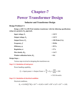
1. Chapter-7
Power Transformer Design
Inductor and Transformer Design
Design Problem # 1
Design a (250 VA) 250 Watt isolation transformer with the following specifications
using core geometry 𝑲 𝒈 approach.
Input voltage, 𝑽𝒊 = 115 V
Output voltage, 𝑽 𝒐 = 115 V
Output Power, 𝑷 𝒐 = 250 Watts (VA)
Frequency, 𝒇 = 50 Hz
Efficiency, 𝜼 = 95 %
Regulation, 𝜶 = 5 %
Flux density, 𝑩 𝒂𝒄 = 1.6 T
Window utilization factor, 𝑲 𝒖 = 0.4
Design Steps: -
Various steps involved in designing this transformer are:
Step # 1: Calculation of total power
Power handling capability,
𝑃𝑡 = 𝐼𝑛𝑝𝑢𝑡 𝑝𝑜𝑤𝑒𝑟 + 𝑂𝑢𝑡𝑝𝑢𝑡 𝑃𝑜𝑤𝑒𝑟 =
𝑃𝑂
𝜂
+ 𝑃𝑂 =
250
0.95
+ 250
= 513.16 𝑤𝑎𝑡𝑡𝑠.
Step # 2: Calculation of electrical condition
Electrical conditions,
𝐾𝑒 = 0.145𝐾𝑓
2
𝑓2
𝐵 𝑚
2
× 10−4
= 0.145 × 4.442
× 502
× 1.62
× 10−4
= 1.83.

2. Step # 3: Calculation of core geometry
Core geometry,
𝐾𝑔 =
𝑃𝑡
2𝐾 𝑒 𝛼
=
513.16
2×1.83×5
= 𝟐𝟖. 𝟎𝟒 cm5
.
Step # 4: Selection of transformer core
For the core geometry calculated in step # 3, the closest lamination number is 𝑬𝑰 − 𝟏𝟓𝟎.
Table 7.1 Design data for EI laminations
Part
No.
Wtcu in
gm
Wtfe in
gm
MLT
in cm
MPL
in cm
Wa/Ac Ac in
cm2
Wa in
cm2
Ap in
cm4
Kg in
cm5
At in
cm2
EI-150 853 2334 22 22.9 0.789 13.79 10.887 150.136 37.579 479
Table 3.2 Dimensional data for EI laminations.

3. E
D
D
Figure 7.1 EI-laminations and dimensions of different parts.
For 𝑬𝑰 − 𝟏𝟓𝟎 lamination,
Magnetic path length (MPL) = 22.9 cm
Core weight = 2334 gm
Copper weight = 853 gm
Mean length turn (MLT) = 22 cm
Iron area, 𝐴 𝑐 = 13.8 cm2
Window area, 𝑊𝑎 = 10.89 cm2
Area product, 𝐴 𝑝 = 𝐴 𝑐 × 𝑊𝑎 = 150 cm2
Core geometry, 𝐾𝑔 = 28.04 cm5
Surface area, 𝐴 𝑡 = 479 cm2
Step # 5: Calculation of primary number of turns
Primary number of turns,
𝑁𝑝 =
𝑉𝑖×104
𝐾 𝑓 𝐵 𝑎𝑐 𝑓𝐴 𝑐
=
115×104
4.44×1.6×50×13.8
= 234.6 = 𝟐𝟑𝟓 turns.
Step # 6: Calculation of current density
Current density,
𝐽 =
𝑃𝑡×104
𝐾 𝑓×𝐾 𝑢×𝐵 𝑎𝑐×𝑓×𝐴 𝑝
=
513.16×104
4.44×0.4×1.6×50×150
= 240.78 A/cm2
.
Step # 7: Calculation of input current
Input current,
𝐼𝑖 =
𝑖𝑛𝑝𝑢𝑡 𝑝𝑜𝑤𝑒𝑟
𝑖𝑛𝑝𝑢𝑡 𝑣𝑜𝑙𝑡𝑎𝑔𝑒
=
𝑃𝑜/𝜂
𝑉𝑖
=
(
250
0.95
)
115
= 2.288 A.

4. Step # 8: Calculation of cross-sectional area (bare) of conductor for primary winding
Bare conductor cross-sectional area,
𝐴 𝑤𝑝(𝐵) =
𝐼 𝑖
𝐽
=
2.288
240.78
= 0.0095 cm2
= 0.95 𝑚𝑚2
.
Step # 9: Selection of wire from wire table
The closest Standard Wire Gauge (SWG) corresponding to the bare conductor area
calculated in step # 8 is 18 SWG.
For 18 SWG conductor,
𝐴 𝑤𝑝(𝐵) = 1.17 mm2
.
Resistance for 18 SWG conductor is 14.8
Ω
Km
= 148
𝜇Ω
𝑐𝑚
.
Step # 10: Calculation of primary winding resistance
Resistance of primary winding,
𝑅 𝑝 = 𝑀𝐿𝑇 × 𝑁𝑝 × 148 × 10−6
= 22 × 235 × 148 × 10−6
= 0.765 Ω.
Step # 11: Calculation of copper loss in primary winding
Primary winding copper loss
𝑃𝑝 = 𝐼 𝑝
2
× 𝑅 𝑝 = 2.2882
× 0.765 = 4 Watts.
Step # 12: Calculation of secondary winding turns
Number of turns in the secondary winding
𝑁𝑠 =
𝑁 𝑝×𝑉𝑠
𝑉𝑖
[1 +
𝛼
100
] =
235×115
115
[1 +
5
100
] = 247.

5. Step # 13: Calculation of bare conductor area for secondary winding
Cross-sectional area of bare conductor for secondary winding
𝐴 𝑤𝑠(𝐵) =
𝐼 𝑜
𝐽
=
2.17
240.78
= 0.00901 cm2
= 0.901 mm2
.
Step # 14: Selection of conductor size required for secondary winding
From the wire table, the closest cross-sectional area (i.e. next to) is found by choosing the
conductor size as 18 SWG.
For 18 SWG wire, bare conductor area is 1.17 mm2
, for which resistance/cm is 148 𝜇Ω/𝑐𝑚.
Step # 15: Calculation of secondary winding resistance
Secondary winding resistance
𝑅 𝑠 = 𝑀𝐿𝑇 × 𝑁𝑠 × 148 × 10−6
= 22 × 247 × 148 × 10−6
= 0.804 Ω.
Step # 16: Calculation of copper in secondary winding
Copper loss in secondary winding,
𝑃𝑠 = 𝐼 𝑜
2
× 𝑅 𝑠 = 2.172
× 0.804 = 3.8 Watts.
Step # 17: Calculation of total copper loss
Total copper loss,
𝑃𝑐𝑢 = 𝑃𝑝 + 𝑃𝑠 = 4 + 3.8 = 7.8 Watts.
Step # 18: Calculation of voltage regulation
Voltage regulation,
𝛼 =
𝑃𝑐𝑢
𝑃𝑜
=
7.8
250
= 0.0312 = 3.12 %.
Step # 19: Calculation of Watts per Kg (W/K)
Watts/Kg,
𝑊
𝐾
= 0.000557𝑓1.68
𝐵𝑎𝑐
1.86
= 0.000557 × 501.68
× 1.61.86
= 0.9545.
Step # 20: Calculation of core loss
Core loss,
𝑃𝑓𝑒 =
𝑊
𝐾
× 𝑊𝑡𝑓𝑒 × 10−3
= 0.9545 × 2334 × 10−3
= 2.23 Watts.

6. Step # 21: Calculation of total loss
Total loss in the transformer,
𝑃Σ = 𝑃𝑐𝑢 + 𝑃𝑓𝑒 = 7.8 + 2.23 = 10.03 Watts.
Step # 22: Calculation of Watts/unit area
Watts/unit area,
𝜓 =
𝑃Σ
𝐴 𝑡
=
10.03
479
= 0.021 Watts/cm2
.

7. Step # 23: Calculation of temperature rise
Temperature rise,
𝑇𝑟 = 450𝜓0.826
= 450 × 0.0210.826
= 18.51 0
C.
Step # 24: Calculation of window utilization factor
Window utilization factor,
𝐾 𝑢 = 𝐾 𝑢𝑝 + 𝐾 𝑢𝑠 =
𝑁 𝑝×𝐴 𝑤𝑝(𝐵)
𝑊𝑎
+
𝑁 𝑠×𝐴 𝑤𝑠(𝐵)
𝑊𝑎
=
235×0.0117+247×0.0117
10.89
= 0.52.