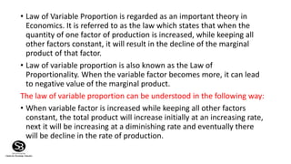
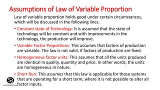
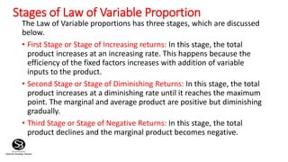
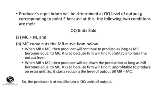
Dr. C.V. Suresh Babu
Variable
Proportion
of
• Law of Variable Proportion is regarded as an important theory in
Economics. It is referred to as the law which states that when the
quantity of one factor of production is increased, while keeping all
other factors constant, it will result in the decline of the marginal
product of that factor.
• Law of variable proportion is also known as the Law of
Proportionality. When the variable factor becomes more, it can lead
to negative value of the marginal product.
The law of variable proportion can be understood in the following way:
• When variable factor is increased while keeping all other factors
constant, the total product will increase initially at an increasing rate,
next it will be increasing at a diminishing rate and eventually there
will be decline in the rate of production.
Assumptions of Law of Variable Proportion
Law of variable proportion holds good under certain circumstances,
which will be discussed in the following lines.
• Constant state of Technology: It is assumed that the state of
technology will be constant and with improvements in the
technology, the production will improve.
• Variable Factor Proportions: This assumes that factors of production
are variable. The law is not valid, if factors of production are fixed.
• Homogeneous factor units: This assumes that all the units produced
are identical in quality, quantity and price. In other words, the units
are homogeneous in nature.
• Short Run: This assumes that this law is applicable for those systems
that are operating for a short term, where it is not possible to alter all
factor inputs.
Stages of Law of Variable Proportion
The Law of Variable proportions has three stages, which are discussed
below.
• First Stage or Stage of Increasing returns: In this stage, the total
product increases at an increasing rate. This happens because the
efficiency of the fixed factors increases with addition of variable
inputs to the product.
• Second Stage or Stage of Diminishing Returns: In this stage, the total
product increases at a diminishing rate until it reaches the maximum
point. The marginal and average product are positive but diminishing
gradually.
• Third Stage or Stage of Negative Returns: In this stage, the total
product declines and the marginal product becomes negative.
• Producer’s equilibrium will be determined at OQ level of output g
corresponding to point E because at this, the following two conditions
are met:
OQ Units Sold
(a) MC = M, and
(b) MC curve cuts the MR curve from below.
• When MR > MC, then producer will continue to produce as long as MR
becomes equal to MC. It is so because firm will find it profitable to raise the
output level.
• When MR < MC, then producer will cut down the production as long as MR
becomes equal to MC. It is so because firm will find it Unprofitable to produce
an extra unit. So, it starts reducing the level of output till MR = MC.
So, the producer is at equilibrium at OQ units of output.
For our example, we are assuming that labour is a variable factor. Hence, we
have following table-
We are increasing the total number of labours working on a machine. Remember that we can't
afford to buy a new machine as we are in the short run, but we can surely increase the number
of labours working on the machine. Hence, we gradually increase the labour from one to eleven.
From the table above, we can observe the following:
• The Total Product increases with increase in labour but later it falls.
• The Average product too increases initially and later starts falling.
• The Marginal Product also increases initially but later falls.
• Now if we concentrate only on the Marginal product, we will understand that the 1st labor has produced
100 units but the 2nd has produced 110 units and the third has produced even more i.e.130 units. But the
question arises why? why it so happens that the second and third labours are producing more than the first?
• It happens because of ‘division of labour’. As the number of labours are increasing on a machine, the
efficiency of the new labour will increase initially because of division of work.
• In sports like cricket too something similar happens more often. The batsman at number 3 generally scores
more than the batsman at number 1 position. This happens because when the batsmen at number one and
two position open the innings, they set a good platform for the batsman at number 3 position to score more.
• If we observe the behavior of the marginal product further, we would know that it is gradually falling. Hence,
the new worker is producing lesser units than the earlier one. But why does this happen? What makes the
new worker produce less? Won’t the division of work apply here?
• The answer to this is that, as the number of workers are increasing, there is very little work left for the new
worker to do on the machine. Hence, the end workers have very little to contribute as already maximum
work is done by the initial workers.
• Comparing thus with cricket again, the tailenders will contribute to the score of a team but their
contribution will be negligible. This is because, they don’t have much overs to play in a limited overs game.
• Also, the marginal product of the 11th labour is negative. This would clearly imply that the 11th labour is not
needed. The machine in the example can only have a maximum of 10 labours. Hence, if there is excess
labour, this would create a havoc and the disturbance would cause the ‘Total Product’ to fall instead of
rising.
• Hence, a prudent entrepreneur stops at the end of stage 2 as shown in the table where the ‘Total Product’ is
maximum and the ‘Marginal Product’ is zero.
Understanding the stages:
• This is how the graph looks like-
1.Stage 1- Law of increasing returns: Here, the total
product increases at a faster rate. The marginal product
increases and then falls. The average product increases
and reaches its maximum point.
2.Stage 2- Law of diminishing returns: Here, the total
product increases at a slower rate and reaches its
maximum point. The average product falls for the very first
time.
3.Stage 3- Law of negative returns: Here, the total
product falls for the very first time. The average product
falls further and the marginal product goes negative for
the very first time.

Law of variable proportion

  • 1.
    Dr. C.V. SureshBabu Variable Proportion of
  • 2.
    • Law ofVariable Proportion is regarded as an important theory in Economics. It is referred to as the law which states that when the quantity of one factor of production is increased, while keeping all other factors constant, it will result in the decline of the marginal product of that factor. • Law of variable proportion is also known as the Law of Proportionality. When the variable factor becomes more, it can lead to negative value of the marginal product. The law of variable proportion can be understood in the following way: • When variable factor is increased while keeping all other factors constant, the total product will increase initially at an increasing rate, next it will be increasing at a diminishing rate and eventually there will be decline in the rate of production.
  • 3.
    Assumptions of Lawof Variable Proportion Law of variable proportion holds good under certain circumstances, which will be discussed in the following lines. • Constant state of Technology: It is assumed that the state of technology will be constant and with improvements in the technology, the production will improve. • Variable Factor Proportions: This assumes that factors of production are variable. The law is not valid, if factors of production are fixed. • Homogeneous factor units: This assumes that all the units produced are identical in quality, quantity and price. In other words, the units are homogeneous in nature. • Short Run: This assumes that this law is applicable for those systems that are operating for a short term, where it is not possible to alter all factor inputs.
  • 4.
    Stages of Lawof Variable Proportion The Law of Variable proportions has three stages, which are discussed below. • First Stage or Stage of Increasing returns: In this stage, the total product increases at an increasing rate. This happens because the efficiency of the fixed factors increases with addition of variable inputs to the product. • Second Stage or Stage of Diminishing Returns: In this stage, the total product increases at a diminishing rate until it reaches the maximum point. The marginal and average product are positive but diminishing gradually. • Third Stage or Stage of Negative Returns: In this stage, the total product declines and the marginal product becomes negative.
  • 5.
    • Producer’s equilibriumwill be determined at OQ level of output g corresponding to point E because at this, the following two conditions are met: OQ Units Sold (a) MC = M, and (b) MC curve cuts the MR curve from below. • When MR > MC, then producer will continue to produce as long as MR becomes equal to MC. It is so because firm will find it profitable to raise the output level. • When MR < MC, then producer will cut down the production as long as MR becomes equal to MC. It is so because firm will find it Unprofitable to produce an extra unit. So, it starts reducing the level of output till MR = MC. So, the producer is at equilibrium at OQ units of output.
  • 6.
    For our example,we are assuming that labour is a variable factor. Hence, we have following table- We are increasing the total number of labours working on a machine. Remember that we can't afford to buy a new machine as we are in the short run, but we can surely increase the number of labours working on the machine. Hence, we gradually increase the labour from one to eleven.
  • 7.
    From the tableabove, we can observe the following: • The Total Product increases with increase in labour but later it falls. • The Average product too increases initially and later starts falling. • The Marginal Product also increases initially but later falls.
  • 8.
    • Now ifwe concentrate only on the Marginal product, we will understand that the 1st labor has produced 100 units but the 2nd has produced 110 units and the third has produced even more i.e.130 units. But the question arises why? why it so happens that the second and third labours are producing more than the first? • It happens because of ‘division of labour’. As the number of labours are increasing on a machine, the efficiency of the new labour will increase initially because of division of work. • In sports like cricket too something similar happens more often. The batsman at number 3 generally scores more than the batsman at number 1 position. This happens because when the batsmen at number one and two position open the innings, they set a good platform for the batsman at number 3 position to score more. • If we observe the behavior of the marginal product further, we would know that it is gradually falling. Hence, the new worker is producing lesser units than the earlier one. But why does this happen? What makes the new worker produce less? Won’t the division of work apply here? • The answer to this is that, as the number of workers are increasing, there is very little work left for the new worker to do on the machine. Hence, the end workers have very little to contribute as already maximum work is done by the initial workers. • Comparing thus with cricket again, the tailenders will contribute to the score of a team but their contribution will be negligible. This is because, they don’t have much overs to play in a limited overs game. • Also, the marginal product of the 11th labour is negative. This would clearly imply that the 11th labour is not needed. The machine in the example can only have a maximum of 10 labours. Hence, if there is excess labour, this would create a havoc and the disturbance would cause the ‘Total Product’ to fall instead of rising. • Hence, a prudent entrepreneur stops at the end of stage 2 as shown in the table where the ‘Total Product’ is maximum and the ‘Marginal Product’ is zero.
  • 9.
    Understanding the stages: •This is how the graph looks like- 1.Stage 1- Law of increasing returns: Here, the total product increases at a faster rate. The marginal product increases and then falls. The average product increases and reaches its maximum point. 2.Stage 2- Law of diminishing returns: Here, the total product increases at a slower rate and reaches its maximum point. The average product falls for the very first time. 3.Stage 3- Law of negative returns: Here, the total product falls for the very first time. The average product falls further and the marginal product goes negative for the very first time.