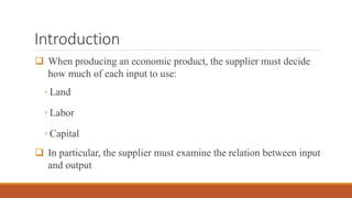
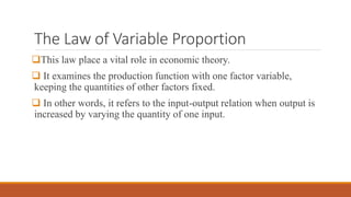
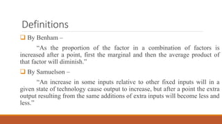
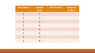
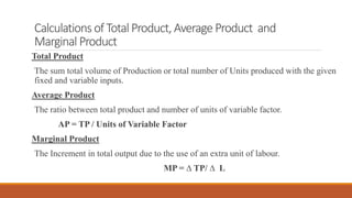
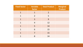
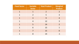
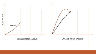
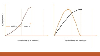
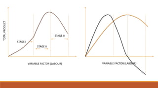
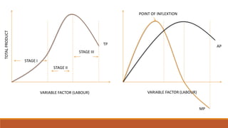
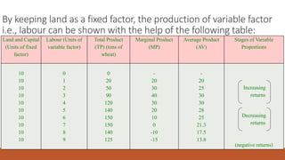
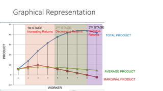
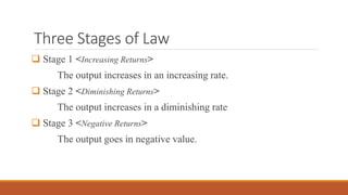
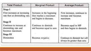
Law of Variable
Proportion
PRESENTED BY
DHRUBAJYOTI SADHUKHAN
CONTENTS
1. INTRODUCTION
2. DEFINITION
3. ASSUMPTION
4. EXPLAINATION
I. TABULATION METHOD
II. GRAPHICAL METHOD
5. THREE STAGES OF LAW
6. CAUSES
Introduction
 When producing an economic product, the supplier must decide
how much of each input to use:
◦ Land
◦ Labor
◦ Capital
 In particular, the supplier must examine the relation between input
and output
The Law of Variable Proportion
This law place a vital role in economic theory.
 It examines the production function with one factor variable,
keeping the quantities of other factors fixed.
 In other words, it refers to the input-output relation when output is
increased by varying the quantity of one input.
Definitions
 By Benham –
“As the proportion of the factor in a combination of factors is
increased after a point, first the marginal and then the average product of
that factor will diminish.”
 By Samuelson –
“An increase in some inputs relative to other fixed inputs will in a
given state of technology cause output to increase, but after a point the extra
output resulting from the same additions of extra inputs will become less and
less.”
By Leftwitch –
“The law of variable proportion states that if the inputs of one
resource is increased by equal increment per unit of time while the
inputs of other resources are held constant, total output will increase,
but beyond some point the resulting output increases will become
smaller and smaller.”
Assumptions
(i) Constant Technology:
The state of technology is assumed to be given and constant. If there
is an improvement in technology the production function will move
upward.
(ii) Factor Proportions are Variable:
The law assumes that factor proportions are variable. If factors of
production are to be combined in a fixed proportion, the law has no
validity.
(iii) Homogeneous Factor Units:
The units of variable factor are homogeneous. Each unit is identical
in quality and amount with every other unit.
(iv) Short-Run:
The law operates in the short-run where it is not possible to vary all
factor inputs.
Assumptions
Explanation of the law
 In order to understand the law of variable proportion, we take the
example of agriculture. Suppose land and labour are the only two
factors of production.
 As we can observe from the table (next slide), the output varies with
one of the input is fixed and varying other input.
 The output varies in three different stages.
Fixed factor Variable
factor
Total Product Marginal
Product
1 1
1 2
1 3
1 4
1 5
1 6
1 7
1 8
Calculations ofTotalProduct, Average Product and
Marginal Product
Total Product
The sum total volume of Production or total number of Units produced with the given
fixed and variable inputs.
Average Product
The ratio between total product and number of units of variable factor.
AP = TP / Units of Variable Factor
Marginal Product
The Increment in total output due to the use of an extra unit of labour.
MP = ∆ TP/ ∆ L
Fixed factor Variable
factor
Total Product Marginal
Product
1 1 2
1 2 5
1 3 9
1 4 12
1 5 14
1 6 15
1 7 15
1 8 14
Fixed factor Variable
factor
Total Product Marginal
Product
1 1 2 2
1 2 5 3
1 3 9 4
1 4 12 3
1 5 14 2
1 6 15 1
1 7 15 0
1 8 14 -1
VARIABLE FACTOR (LABOUR) VARIABLE FACTOR (LABOUR)
TOTALPRODUCT
STAGE I
VARIABLE FACTOR (LABOUR) VARIABLE FACTOR (LABOUR)
TOTALPRODUCT
STAGE I STAGE II
VARIABLE FACTOR (LABOUR) VARIABLE FACTOR (LABOUR)
TOTALPRODUCT
STAGE III
STAGE I
STAGE II
STAGE III
POINT OF INFLEXTION
STAGE I
STAGE II
TP AP
MP
VARIABLE FACTOR (LABOUR) VARIABLE FACTOR (LABOUR)
TOTALPRODUCT
By keeping land as a fixed factor, the production of variable factor
i.e., labour can be shown with the help of the following table:
Land and Capital
(Units of fixed
factor)
Labour (Units of
variable factor)
Total Product
(TP) (tons of
wheat)
Marginal Product
(MP)
Average Product
(AV)
Stages of Variable
Proportions
10
10
10
10
10
10
10
10
10
10
0
1
2
3
4
5
6
7
8
9
0
20
50
90
120
140
150
150
140
125
-
20
30
40
30
20
10
0
-10
-15
-
20
25
30
30
28
25
21.3
17.5
13.8
Increasing
returns
Decreasing
returns
(negative returns)
Graphical Representation
TOTAL PRODUCT
AVERAGE PRODUCT
MARGINAL PRODUCT
WORKER
PRODUCT
1st STAGE
Increasing Returns
2ND STAGE
Decreasing Returns
3RD STAGE
Negative
Returns
Three Stages of Law
 Stage 1 <Increasing Returns>
The output increases in an increasing rate.
 Stage 2 <Diminishing Returns>
The output increases in a diminishing rate
 Stage 3 <Negative Returns>
The output goes in negative value.
Cause of Increasing Returns
 Under Utilization of Fixed Factor:
In initial stage of production, fixed factors of production like
land or machine, is under-utilized. More units of variable
factor, like labour, are needed for its proper utilization. As a
result of employment of additional units of variable factors
there is proper utilization of fixed factor.
In short, increasing returns to a factor begins to manifest
itself in the first stage.
Cause of Diminishing Returns
 Fixed Factors of Production:
Some of the factors of production are fixed during the short
period.
When the fixed factor is used with variable factor, then its
ratio compared to variable factor falls. Production is the
result of the co-operation of all factors.
When an additional unit of a variable factor has to produce
with the help of relatively fixed factor, then the marginal
return of variable factor begins to decline.
Optimum Production:
After making the optimum use of a fixed factor, then the
marginal return of such variable factor begins to diminish.
The simple reason is that after the optimum use, the ratio of
fixed and variable factors become defective.
Let us suppose a machine is a fixed factor of production. It
is put to optimum use when 4 labourers are employed on it.
If 5 labourers are put on it, then total production increases
very little and the marginal product diminishes.
Imperfect Substitutes:
Mrs. Joan Robinson has put the argument that imperfect
substitution of factors is mainly responsible for the operation of
the law of diminishing returns. One factor cannot be used in
place of the other factor.
After optimum use of fixed factors, variable factors are
increased and the amount of fixed factor could be increased by
its substitutes.
Such a substitution would increase the production in the same proportion as
earlier. But in real practice factors are imperfect substitutes. However, after
the optimum use of a fixed factor, it cannot be substituted by another factor.
Cause of Negative Returns
 “too many cooks spoil the broth”
 When a business experiences decreasing returns and the quantity of
variable factor is further increased, the marginal returns becomes
negative.
In this phase, with every successive increase in the quantity of
variable factor employed, the additional returns are negative and
therefore the total returns start diminishing.
 The marginal product of the variable factor is negative due to
‘Excessiveness’.
THANK YOU

Law of variable proportion

  • 1.
    Law of Variable Proportion PRESENTEDBY DHRUBAJYOTI SADHUKHAN
  • 2.
    CONTENTS 1. INTRODUCTION 2. DEFINITION 3.ASSUMPTION 4. EXPLAINATION I. TABULATION METHOD II. GRAPHICAL METHOD 5. THREE STAGES OF LAW 6. CAUSES
  • 3.
    Introduction  When producingan economic product, the supplier must decide how much of each input to use: ◦ Land ◦ Labor ◦ Capital  In particular, the supplier must examine the relation between input and output
  • 4.
    The Law ofVariable Proportion This law place a vital role in economic theory.  It examines the production function with one factor variable, keeping the quantities of other factors fixed.  In other words, it refers to the input-output relation when output is increased by varying the quantity of one input.
  • 5.
    Definitions  By Benham– “As the proportion of the factor in a combination of factors is increased after a point, first the marginal and then the average product of that factor will diminish.”  By Samuelson – “An increase in some inputs relative to other fixed inputs will in a given state of technology cause output to increase, but after a point the extra output resulting from the same additions of extra inputs will become less and less.”
  • 6.
    By Leftwitch – “Thelaw of variable proportion states that if the inputs of one resource is increased by equal increment per unit of time while the inputs of other resources are held constant, total output will increase, but beyond some point the resulting output increases will become smaller and smaller.”
  • 7.
    Assumptions (i) Constant Technology: Thestate of technology is assumed to be given and constant. If there is an improvement in technology the production function will move upward. (ii) Factor Proportions are Variable: The law assumes that factor proportions are variable. If factors of production are to be combined in a fixed proportion, the law has no validity.
  • 8.
    (iii) Homogeneous FactorUnits: The units of variable factor are homogeneous. Each unit is identical in quality and amount with every other unit. (iv) Short-Run: The law operates in the short-run where it is not possible to vary all factor inputs. Assumptions
  • 9.
    Explanation of thelaw  In order to understand the law of variable proportion, we take the example of agriculture. Suppose land and labour are the only two factors of production.  As we can observe from the table (next slide), the output varies with one of the input is fixed and varying other input.  The output varies in three different stages.
  • 10.
    Fixed factor Variable factor TotalProduct Marginal Product 1 1 1 2 1 3 1 4 1 5 1 6 1 7 1 8
  • 11.
    Calculations ofTotalProduct, AverageProduct and Marginal Product Total Product The sum total volume of Production or total number of Units produced with the given fixed and variable inputs. Average Product The ratio between total product and number of units of variable factor. AP = TP / Units of Variable Factor Marginal Product The Increment in total output due to the use of an extra unit of labour. MP = ∆ TP/ ∆ L
  • 12.
    Fixed factor Variable factor TotalProduct Marginal Product 1 1 2 1 2 5 1 3 9 1 4 12 1 5 14 1 6 15 1 7 15 1 8 14
  • 13.
    Fixed factor Variable factor TotalProduct Marginal Product 1 1 2 2 1 2 5 3 1 3 9 4 1 4 12 3 1 5 14 2 1 6 15 1 1 7 15 0 1 8 14 -1
  • 14.
    VARIABLE FACTOR (LABOUR)VARIABLE FACTOR (LABOUR) TOTALPRODUCT STAGE I
  • 15.
    VARIABLE FACTOR (LABOUR)VARIABLE FACTOR (LABOUR) TOTALPRODUCT STAGE I STAGE II
  • 16.
    VARIABLE FACTOR (LABOUR)VARIABLE FACTOR (LABOUR) TOTALPRODUCT STAGE III STAGE I STAGE II
  • 17.
    STAGE III POINT OFINFLEXTION STAGE I STAGE II TP AP MP VARIABLE FACTOR (LABOUR) VARIABLE FACTOR (LABOUR) TOTALPRODUCT
  • 18.
    By keeping landas a fixed factor, the production of variable factor i.e., labour can be shown with the help of the following table: Land and Capital (Units of fixed factor) Labour (Units of variable factor) Total Product (TP) (tons of wheat) Marginal Product (MP) Average Product (AV) Stages of Variable Proportions 10 10 10 10 10 10 10 10 10 10 0 1 2 3 4 5 6 7 8 9 0 20 50 90 120 140 150 150 140 125 - 20 30 40 30 20 10 0 -10 -15 - 20 25 30 30 28 25 21.3 17.5 13.8 Increasing returns Decreasing returns (negative returns)
  • 19.
    Graphical Representation TOTAL PRODUCT AVERAGEPRODUCT MARGINAL PRODUCT WORKER PRODUCT 1st STAGE Increasing Returns 2ND STAGE Decreasing Returns 3RD STAGE Negative Returns
  • 20.
    Three Stages ofLaw  Stage 1 <Increasing Returns> The output increases in an increasing rate.  Stage 2 <Diminishing Returns> The output increases in a diminishing rate  Stage 3 <Negative Returns> The output goes in negative value.
  • 22.
    Cause of IncreasingReturns  Under Utilization of Fixed Factor: In initial stage of production, fixed factors of production like land or machine, is under-utilized. More units of variable factor, like labour, are needed for its proper utilization. As a result of employment of additional units of variable factors there is proper utilization of fixed factor. In short, increasing returns to a factor begins to manifest itself in the first stage.
  • 23.
    Cause of DiminishingReturns  Fixed Factors of Production: Some of the factors of production are fixed during the short period. When the fixed factor is used with variable factor, then its ratio compared to variable factor falls. Production is the result of the co-operation of all factors. When an additional unit of a variable factor has to produce with the help of relatively fixed factor, then the marginal return of variable factor begins to decline.
  • 24.
    Optimum Production: After makingthe optimum use of a fixed factor, then the marginal return of such variable factor begins to diminish. The simple reason is that after the optimum use, the ratio of fixed and variable factors become defective. Let us suppose a machine is a fixed factor of production. It is put to optimum use when 4 labourers are employed on it. If 5 labourers are put on it, then total production increases very little and the marginal product diminishes.
  • 25.
    Imperfect Substitutes: Mrs. JoanRobinson has put the argument that imperfect substitution of factors is mainly responsible for the operation of the law of diminishing returns. One factor cannot be used in place of the other factor. After optimum use of fixed factors, variable factors are increased and the amount of fixed factor could be increased by its substitutes. Such a substitution would increase the production in the same proportion as earlier. But in real practice factors are imperfect substitutes. However, after the optimum use of a fixed factor, it cannot be substituted by another factor.
  • 26.
    Cause of NegativeReturns  “too many cooks spoil the broth”  When a business experiences decreasing returns and the quantity of variable factor is further increased, the marginal returns becomes negative. In this phase, with every successive increase in the quantity of variable factor employed, the additional returns are negative and therefore the total returns start diminishing.  The marginal product of the variable factor is negative due to ‘Excessiveness’.
  • 27.