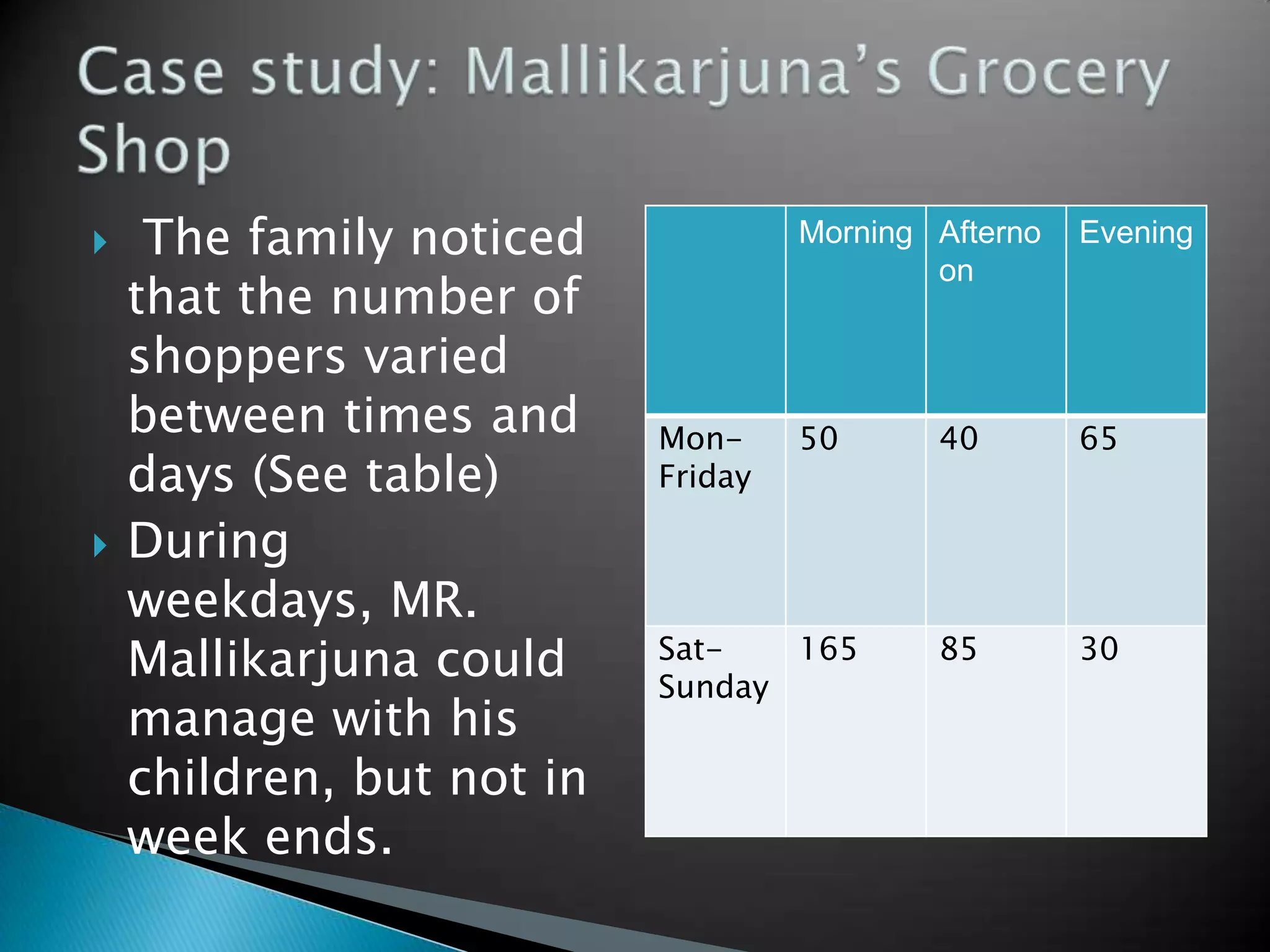
Here are the key points regarding Mallikarjuna's problem and suggestions to improve the functioning of the shop: 1. Mallikarjuna's problem fits the law of variable proportions. As he increases the number of assistants (variable input) from 0 to 3, total output/customers served initially increases at an increasing rate as one assistant can help multiple customers. However, beyond 3 assistants, adding more in the limited space leads to diminishing returns as customers get inconvenienced in the crowded shop. 2. Suggestions to improve: - Increase shop floor area to accommodate more customers comfortably without overcrowding. This allows employing more assistants without diminishing returns. - Add more billing counters to reduce

2. SUMITTED BY
MUKESH KUMAR
NAWAZ AHAMED
SANDIP
SANTOSH
SACHIN
AMAR

3. Production Function-Explains the
relationship between factor input
and output in physical terms. Or the
term PRODUCTION means
transformation of physical “inputs”
into physical “outputs”.

4.  A production function can be represented in
the form of a mathematical model of
equation as Q = f ( a,b,c,…… etc.) where Q
stands for quantity of output per unit of time
and a, b, c, etc are the various factor inputs
like land, capital, labour etc, which are used
in the production of output.

5.  FIXED INPUTS :
 Fixed inputs are those
factors the quantity of which
remains constant irrespective
of the level of output produced
by a firm. For
example, land, buildings, mach
ines, tools, equipments, superi
or types of labour, top
management etc.
 VARIABLE INPUTS :
 Variable inputs are those
factors the quantity of which
varies with variations in the
levels of output produced by a
firm for example, raw
materials, power
fuel, water, transport, labour
and communication etc.

6.  SHORT RUN
 LONG RUN

7. In this case, the producer will keep
all fixed factors as constant and
changes only a few variable factor
inputs. For example, Law of Variable
Proportions.

8. In this case, the producer will vary
the quantities of all factor inputs
both fixed as well as variable in the
same proportion. For example, the
laws of returns to scale.

9. In the short-run the level of production
can be changed by
changing the factor proportions.
This law examines the production
function with on factor variable, keeping
the other factors quantities fixed.

10. The law explains the short-run
production function. When the
quantity of one input is
varied, keeping other inputs
constant, the proportion between
factors changes. When the proportio
n of variable factors
increases, the total output does not
always increase in the
same proportion, but in varying pro
portion.

11.  Only one factor is variable while others are
held constant.
 All units of the variable factor are
homogeneous.
 There is no change in Technology.
 It is possible to vary the proportions in which
different inputs are combined.
 The products are measured in physical units,
i.e., in quintals, tonnes etc.

12. QUANTITY OF TOTAL AVERAGE MARGINAL
LABOUR PRODUCT PRODUCT PRODUCT
(TP) (AP) (MP)
1 100 100 100
2 210 105 110
3 330 110 120
4 430 107.5 100
5 520 104 90
6 600 100 80
7 670 95.7 70
8 720 90 50
9 750 83.3 30
10 760 76 10
11 740 67.2 - 20

13.  It refers to the total volume of goods
produced during a specified period of time.
 Total product (TP)can be raised only by
increasing the quantity of variable factors
employed in production.

14.  Average product can be known by dividing
total product by the total number of units of
the variable factor.
 TP/Q
 Eg- 450/5=90

15.  It is output derived from the employment of
an additional unit of variable factor unit.
 The rate at which total product increases
is known as marginal product.
 Addition to the total product resulting
from a unit increase in the quantity of the vari
able factor.

16.  When AP rises as a result of an increase in the
quantity of variable input, MP is more then
the average product.
 When AP are maximum then MP is equal to
AP. The MP curve cuts the AP curve at its
maximum.
 When AP falls as a result of decrease in
quantity of variable input, MP is less than the
AP.

18.  Stage 1- THE LAW ON INCREASING RETURNS.
 Stage 2- THE LAW OF DIMINSHING RETURNS.
 Stage 3- THE STATE OF NAGATIVE RETURNS

19.  TP increases at an increasing rate up to a
point F.
 MP also rises and is maximum at point F.
 AP goes on rising.
 After point F , TP rises but at diminishing
rate.
 MP falls but is positive.
 Stage 1 ends where AP reaches its highest
point.

20.  TP continues to increase at a diminishing
rate, until it reaches it maximum point H.
 Both MP and AP continuously fall during this
stage.
 Stage ends when TP reaches its maximum
point H.

21.  TP declines.
 MP negative.
 AP is diminishing.

22.  A rational producer will never produce in
stage 3, where MP is negative.
 A rational producer will also not produce in
stage 1, where the MP of fixed factor is
negative.
 The producer producing in stage 1 will not be
making best use of fixed factor and he will
not be utilizing fully the opportunity of
increasing production by increasing quantity
of variable factor.

23.  A rational producer will produce in stage
2, where both MP and AP of variable factors
are diminishing.

25.  Mallikarjuna‟s shop is
very popular and
stocks all kinds of
goods- from rice and
wheat to processed
food, imported
chocolates and cheese.
There is a small
section which has a
photocopying machine
and a STD booth. MR.
Mallikarjuna runs the
shop with the help of
his children.

26.  The family noticed Morning Afterno Evening
on
that the number of
shoppers varied
between times and Mon- 50 40 65
days (See table) Friday
 During
weekdays, MR.
Mallikarjuna could Sat-
Sunday
165 85 30
manage with his
children, but not in
week ends.

27.  Sunday morning buyers were „ value crowd‟-
bulk buyers, spent extra on something new
and attractive but wanted a pleasant
experience and were upset at the
overcrowded shop.
 At certain times there were not many
shoppers.

28. He employed 3 assistants during week
ends, but that did not solve the problem as
the shop had a small floor area and only one
billing machine
1.Can you explain Mallikarjuna‟s problem in
terms of law of variable proportions?
2.Suggest in detail how he can improve the
functioning of the shop.