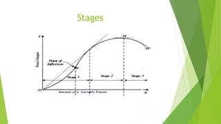
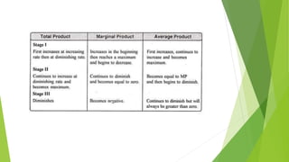
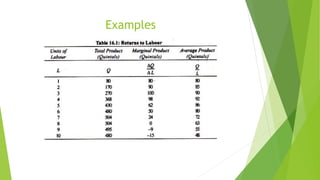
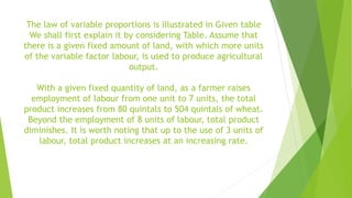
1. The law of variable proportions examines production with one variable input while keeping other inputs fixed. 2. It describes three stages: initially increasing marginal returns, then diminishing marginal returns, and finally negative marginal returns. 3. An example is given of a farmer using increasing amounts of labor on a fixed amount of land, showing total product first rising at an increasing rate, then a diminishing rate, and eventually falling as marginal returns become negative.

1. LAW OF VARIABLE
PROPORTION

2. 1 :- Meaning
2 :- Definition
3 :- Assumption
4 :- Stages
5 :- Examples

3. Meaning
Law of variable proportions occupies an important
place in economic theory. This law examines the
production function with one factor variable, keeping
the quantities of other factors fixed. In other words,
it refers to the input-output relation when output is
increased by varying the quantity of one input.

4. When the quantity of one factor is varied, keeping
the quantity of other factors constant, the
proportion between the variable factor and the
fixed factor is altered; the ratio of employment of
the variable factor to that of the fixed factor goes
on increasing as the quantity of the variable factor
is increased.

5. Definition
[G. Stigler]
As equal increments of one input are added the inputs of
other productive services being held constant, beyond a
certain point the resulting increments of product will
decrease. i.e. the marginal products will diminish
[F. Benham]
As the proportion of one factor in a combination of factors is
increased, after a point first the marginal and then the
average product of that factor will diminish

6. Assumption
1. The state of technology is assumed to be given and
unchanged. If there is improvement in the technology, then
marginal and average products may rise instead of
diminishing.
2. Secondly, there must be some inputs whose quantity is
kept fixed. This is one of the ways by which we can alter the
factor proportions and know its effect on output. This law
does not apply in case all factors are proportionately varied.
Behavior of output as a result of the variation in all inputs is
discussed under ‘returns to scale’

7. 3. Thirdly the law is based upon the possibility of varying the
proportions in which the various factors can be combined to
produce a product. The law does not apply to those cases
where the factors must be used in fixed proportions to yield
a product.

8. Stages

9. 1 :- In this stage, total product curve TP increases at an
increasing rate up to a point. In the Given figure, from the
origin point O to the point F, slope of the total product curve
TP is increasing, that is, up to the point F, the total product
increases at an increasing rate (the total product curve TP is
concave upward up to the point F), which means that the
marginal product MP of the variable factor is rising.

10. 2 :- The total product continues to increase at a diminishing rate
until it reaches its maximum point H where the second stage
ends. In this stage both the marginal product and the average
product of the variable factor are diminishing but remain
positive.
3 :- With the increase in the variable factor the total product
declines and therefore the total product curve TP slopes
downward. As a result, marginal product of the variable factor is
negative and the marginal product curve MP goes below the X-
axis. In this stage the variable factor is too much relative to the
fixed factor. This stage is called the stage of negative returns,
since the marginal product of the variable factor is negative
during this stage.

11. Examples

13. The law of variable proportions is illustrated in Given table
We shall first explain it by considering Table. Assume that
there is a given fixed amount of land, with which more units
of the variable factor labour, is used to produce agricultural
output.
With a given fixed quantity of land, as a farmer raises
employment of labour from one unit to 7 units, the total
product increases from 80 quintals to 504 quintals of wheat.
Beyond the employment of 8 units of labour, total product
diminishes. It is worth noting that up to the use of 3 units of
labour, total product increases at an increasing rate.

14. This fact is clearly revealed from column 3 which shows
successive marginal products of labour as extra units of
labour are used. Marginal product of labour, it may be
recalled, is the increment in total output due to the use of
an extra unit of labour.
It will be seen from Col. 3 of Table. that the marginal
product of labour initially rises and beyond the use of three
units of labour, it starts diminishing. Thus when 3 units of
labour are employed, marginal product of labour is 100 and
with the use of 4th and 5th units of labour marginal product
of labour falls to 98 and 62 respectively.

15. Beyond the use of eight units of labour, total product
diminishes and therefore marginal product of labour
becomes negative. As regards average product of labour, it
rises upto the use of fourth unit of labour and beyond that it
is falling throughout.