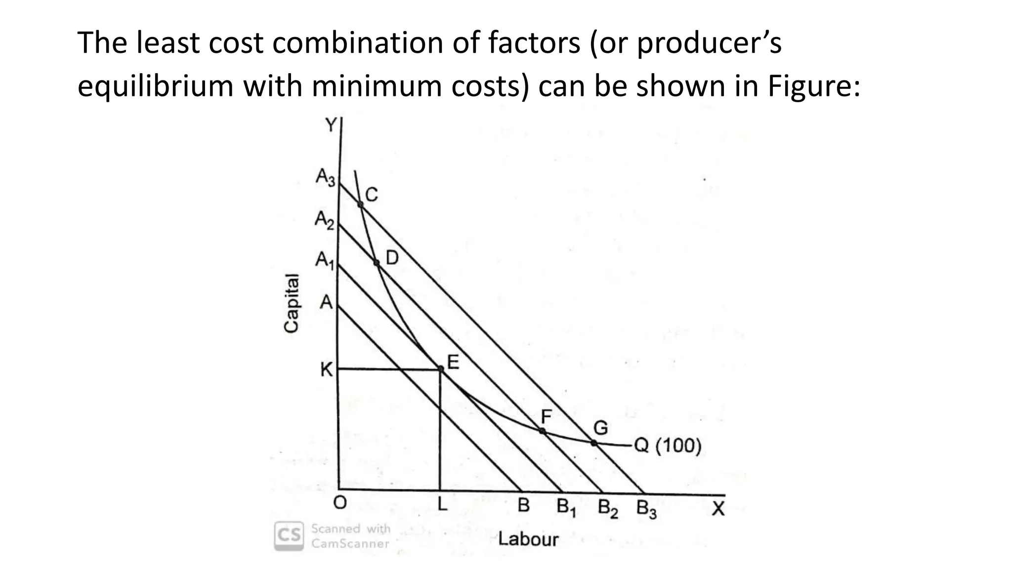
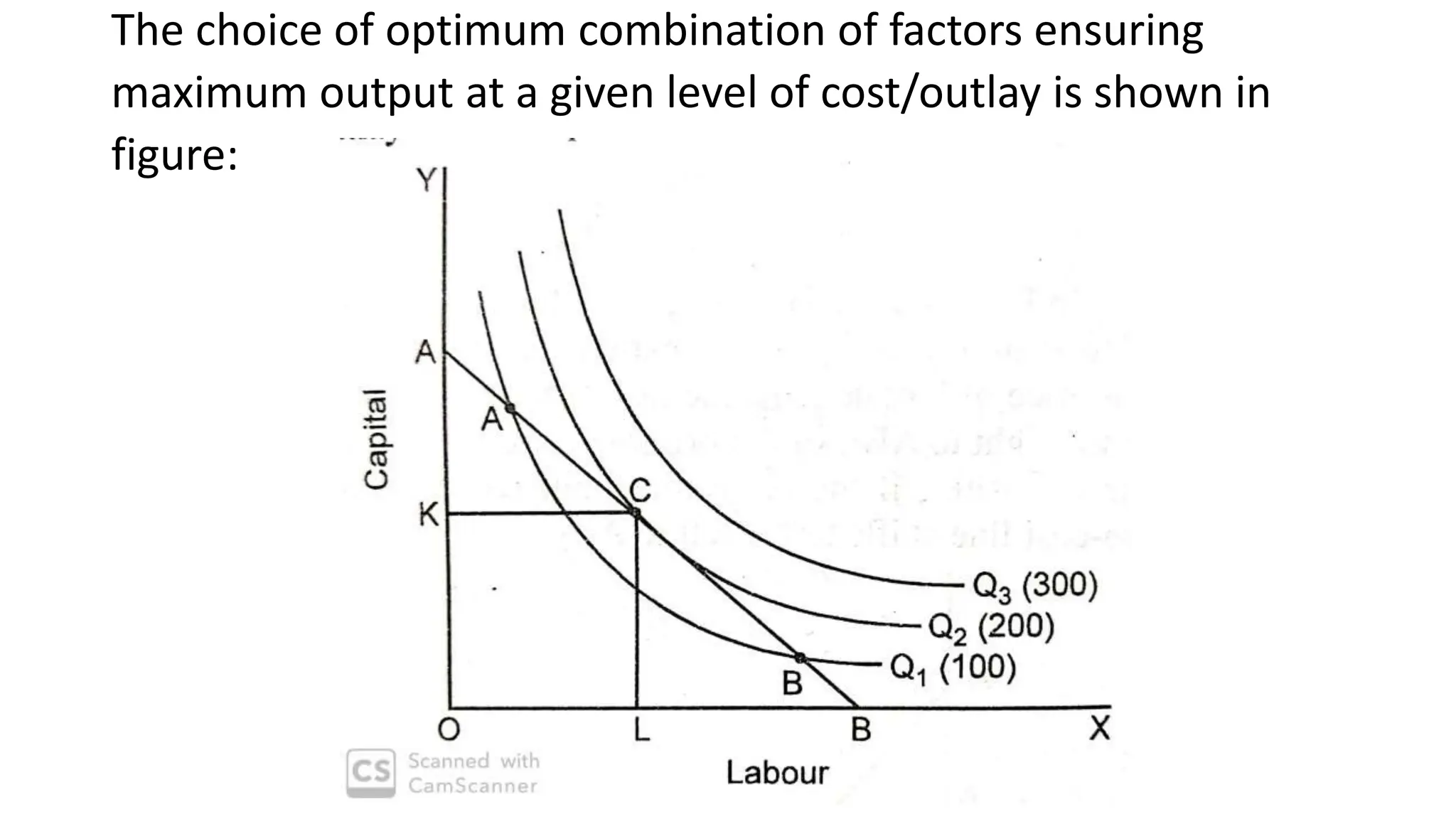
Theory of Production
What is production?
• Production is a process of combining various material inputs and immaterial
inputs (plans, technological know-how) in order to make something for
consumption (output).
• It is the act of creating an output, a good or service which has value and
contributes to the utility of individuals.
• OECD Glossary of Statistical Terms:
“Economic production is an activity carried out under the control and
responsibility of an institutional unit that uses inputs of labour, capital, and
goods and services to produce outputs of goods or services.”
• The area of economics that focuses on production is referred to as
production theory.
What is Production Function?
• The production function is a purely technical relation which connects
factor inputs and outputs.
• It describes the laws of proportion, that is, the transformation of
factor inputs into products (outputs) at any particular time period.
• The production function represents the technology of a firm or of an
industry, or of the economy as a whole.
• The production function includes all the technically efficient methods
of production.
What is Production Function?
• In mathematical terms, the production function can be expressed as:
• Q = f (a, b, c, …n)
• Q = quantity of a commodity produced per unit of time
• a, b, c, … n = physical quantities of productive inputs
Returns to a Factor and Returns to Scale
• In economic theory we are interested in two types of input-output
relations or production functions
• First, we study the production function when the quantities of one
input are varied and quantities of other inputs are kept constant. This
kind of input-output relations forms the subject matter of the law of
variable proportions (or law of diminishing returns or returns to a
factor)
• Second, we study the input-output relations by varying all inputs –
this forms the subject matter of the law of returns to scale
Short-run Production Function:
Returns to a Factor
Production function with one variable input – total,
average and marginal products
Returns to a factor
• In case of a short run production function, some factor inputs remain
fixed while the others can be varied
• Suppose production involves three factor inputs Land (N), Labour (L)
and Capital (K).
• In the short run, land and capital are supposed to remain fixed and
labour alone is a variable factor
• This short run production function can be stated as:
𝑄 = 𝑓(𝐿, 𝐾, 𝑁)
• Returns to a variable factor can be explained through the concepts of
total physical product (TPP), average physical product (APP) and
marginal physical product (MPP)
Total Physical Product (TP)
• The total physical product of a factor means the physical quantities of
total output of a commodity, when a given factor is varied, while
other factors of production remain constant.
• As the input of labour (varying factor) is increased the returns to
factor or the total physical product increase at varying rates.
• Initially the total product increases at an increasing rate, then it increases at a
diminishing/decreasing rate and finally it absolutely declines
Average Physical Product (AP)
• The average physical product of the variable factor (labour) is the
ratio of total physical product to the input of labour employed when
the inputs of capital and land are given (in our example)
• 𝐴𝑃𝐿 =
𝑄
𝐿
• Where Q = TP
• This shows you the production per unit of labour employed
Marginal Physical Product (MP)
• The marginal physical product of the variable factor, labour, is the
additions made to the total physical product through the employment
of an additional (or marginal) unit of labour, the quantities of other
factors remaining constant
• 𝑀𝑃𝐿 =
∆𝑄
∆𝐿
Law of Variable Proportions
I. Meaning
• The law of variable proportions expresses the behaviour of production,
when only one factor input in a combination of factors is varied.
• This law states that given the fixed quantities of other factor inputs, as the
input of one factor, say labour, is increased, the output changes in a non-
proportional way.
• Initially the total product increases at an increasing rate, then it increases
at a diminishing/decreasing rate and finally it absolutely declines
• Also known as the law of non-proportional returns, law of diminishing
returns, law of returns to a factor
Law of variable proportions in the words of Economists:
• George Stigler:
“As equal increments of one input are added, the inputs of other productive
services being held constant, beyond a certain point the resulting increments of
product will decrease, i.e. the marginal products will diminish”
• Behnam:
“As the proportion of one factor in a combination of factors is increased, after a
point, first the marginal and then the average product of that factor will
diminish”
• Paul A Samuelson:
“An increase in some inputs relative to other fixed inputs will, in a given state of
technology, causes output to increase, but after a point the extra output
resulting from the same additions of extra inputs will become less and less”
II. Assumptions
• The law of variable proportions is based upon the following
assumptions:
• 1. The state of technology is given
• 2. One of the factor inputs, say labour, is variable
• 3. The other factor inputs, say land and capital, are fixed
• 4. All the units of variable factor are identical
• 5. The units of variable factor labour are increased one by one
• Suppose a farmer has 20 hectares of land and 2 machines – these are
fixed factor inputs
• Input of labour is increased.
• As the farmer goes on increasing the number of workers one by one,
its effect upon the total, average and marginal physical products is
explained through the Table:
Table 1: Law of Variable Proportions
Input Level Total Physical
Product (in
Quintals)
Average Physical
Product (in
Quintals)
Marginal
Physical Product
(in Quintals)
1 8 8 8
Stage I: Stage of
Increasing Average
Returns
2 20 10 12
3 39 13 19
4 52 13 13
5 60 12 8
Stage II: Stage of
Diminishing Average
Returns
6 66 11 6
7 70 10 4
8 72 9 2
9 72 8 0
10 70 7 -2 Stage III: Stage of
Negative Marginal
Returns
The Law of Variable Proportions
Three stages of the law of variable proportions
• Stage I: State of Increasing
Average Returns
• In this stage the TPP
increases at an increasing
rate until the inflexion
point
• The MPP initially increases
but later declines to 13
quintals
• The APP increases and
approaches the peak level
(13 quintals)
• Stage II: State of Diminishing
Average Returns
• TPP increases at a decreasing
rate
• The APP falls
• MPP also falls until it becomes
equal to zero
• Stage III: Stage of Negative
Marginal Returns
• TPP falls absolutely
• APP continues to fall
• MPP becomes negative
Causes of the Operation of Law of Variable
Proportions:
• Stage I: Stage of increasing average product
• In the beginning as the input of variable factor (labour) is increased, given
the fixed factors, there is an increase in the returns to the fixed factor
• Two reasons for the same:
• 1. Better utilisation of fixed factors
• initially the increase in the variable factor combined with indivisible fixed
factor – better utilisation of indivisible factor
• 2. Specialisation and division of labour
• Stage II and III: the stage of diminishing average product and
negative marginal product
1. Indivisibility of fixed factors
2. Scarcity of skilled variable factor
3. Limited substitution of variable factor for fixed factors
4. Reaching the maximum productive capacity of variable factors
Production Function with two
variable inputs
Production Function with two variable inputs
• two variable inputs - Say for example labour (L) and capital (K)
• analysis of such a production function is based on the fundamental
concept of isoquants or equal product curves.
Isoquant
• The term isoquant is made up of two words
• Iso = equal and
• Quant = quantity
• Isoquant is a curve which represents such combinations of two variable
factor inputs that yield equal output.
• Or
• Isoquant can be defined as the locus of all such combinations of the two
variable factor inputs (say labour and capital) that are capable of producing
the same level of output.
Equal Product Combinations of Labour and Capital
Combinati
ons
Units of
Labour (L)
Units of
Capital (K)
Level of
Output (X)
A 1 24 100
B 2 16 100
C 3 10 100
D 4 6 100
E 5 4 100
Map of Isoquants
Map of Isoquants
• The map of isoquants represents
a series of isoquants indicating
different levels of output from
the different factor
combinations.
• Higher the isoquant, higher is the
level of output and vice-versa
The slop of an isoquant - Marginal Rate of Technical Substitution
• Marginal rate of technical substitution (MRTS) is the rate at which one factor is substituted for the other,
keeping the level of output unchanged.
𝑀𝑅𝑇𝑆𝐿𝐾 =
𝐶ℎ𝑎𝑛𝑔𝑒 𝑖𝑛 𝐶𝑎𝑝𝑖𝑡𝑎𝑙 𝐼𝑛𝑝𝑢𝑡
𝐶ℎ𝑎𝑛𝑔𝑒 𝑖𝑛 𝐿𝑎𝑏𝑜𝑢𝑟 𝑖𝑛𝑝𝑢𝑡
=
𝜕𝐾
𝜕𝐿
• Since all combinations of factors on a given isoquant yield the same level of output, it therefore follows that
• 𝐿𝑜𝑠𝑠 𝑖𝑛 𝑜𝑢𝑡𝑝𝑢𝑡 𝑑𝑢𝑒 𝑡𝑜 𝑟𝑒𝑑𝑢𝑐𝑡𝑖𝑜𝑛 𝑖𝑛 𝑡ℎ𝑒 𝑖𝑛𝑝𝑢𝑡 𝑜𝑓 𝑐𝑎𝑝𝑖𝑡𝑎𝑙 =
𝐺𝑎𝑖𝑛 𝑖𝑛 𝑜𝑢𝑡𝑝𝑢𝑡 𝑑𝑢𝑒 𝑡𝑜 𝑖𝑛𝑐𝑟𝑒𝑎𝑠𝑒 𝑖𝑛 𝑡ℎ𝑒 𝑖𝑛𝑝𝑢𝑡 𝑜𝑓 𝑙𝑎𝑏𝑜𝑢𝑟
− 𝜕𝐾 . 𝑀𝑃𝑃𝐾 = 𝜕𝐿 . 𝑀𝑃𝑃𝐿
−
𝜕𝐾
𝜕𝐿
=
𝑀𝑃𝑃𝐿
𝑀𝑃𝑃𝐾
• therefore,
𝑀𝑅𝑇𝑆𝐿𝐾 =
𝐶ℎ𝑎𝑛𝑔𝑒 𝑖𝑛 𝐶𝑎𝑝𝑖𝑡𝑎𝑙 𝐼𝑛𝑝𝑢𝑡
𝐶ℎ𝑎𝑛𝑔𝑒 𝑖𝑛 𝐿𝑎𝑏𝑜𝑢𝑟 𝑖𝑛𝑝𝑢𝑡
=
𝜕𝐾
𝜕𝐿
=
𝑀𝑃𝑃𝐿
𝑀𝑃𝑃𝐾
Diminishing Marginal Rate of Technical
Substitution
Combinatio
ns
Units of
Labour (L)
Units of
Capital (K)
MRTSLK
A 1 24 -
B 2 16 8:1
C 3 10 6:1
D 4 6 4:1
E 5 4 2:1
• As the producer increases the input of labour
relative to that of capital, there is a fall in the
marginal physical product of labour (MPPL) and a
rise in the marginal physical productivity of capital
(MPPK) on account of the principle of diminishing
returns
• Since
𝑀𝑅𝑇𝑆𝐿𝐾 =
𝑀𝑃𝑃𝐿
𝑀𝑃𝑃𝐾
• a fall in 𝑀𝑃𝑃𝐿 and a rise in 𝑀𝑃𝑃𝐾 leads to decrease
in 𝑀𝑅𝑇𝑆𝐿𝐾 with an increase in the input of labour
Properties of Isoquants
The isoquants or equal product curves have the properties similar to those of
indifference curves of a consumer.
• (i) the isoquants slope negatively or slop
downwards from left to right
• The producer increases the input of one factor and
at the same time reduces the input of other factor
• It is only in such a unique situation that out pf
commodity can remain unchanged.
Properties of Isoquants
The isoquants or equal product curves have the properties similar to those of
indifference curves of a consumer.
• (ii) The isoquants are convex to origin
• (iii) higher the isoquant, higher is the level of
output and vice versa
• iv) Two isoquants cannot cut each other
Shape of isoquants in case of perfect substitutes
Shape of isoquant in case of perfect complements
Optimum Combination of Factors
or
Optimal input combination
or
Producer Equilibrium
• The aim of a rational producer – maximization of profits
• Two ways to realise this aim:
• Minimization of costs, subject to a given output
• Maximization of output subject to a budget constraint
• The factor combination which involves the least cost or maximum profits
signifies an optimum or ideal combination of factors.
• When such a combination is achieved – no incentive for the producer to
make any further change in factor combination – a state of equilibrium
I. Least Cost Combination of Factors
A. Assumptions
1. Producer is rational –wants to secure maximum profits by producing at the
minimum cost
2. Prices of the two varying factors, labour and capital are given
3. All the units of each factor input are identical
4. The factor inputs are divisible
B. Producer Equilibrium Condition
• Given the above assumptions, the equilibrium of producer with the least
cost combination can be determined, if the following condition is met:
• MRTSLK should be equal to the price ratio of labour and capital (where
iso-cost line is tangent to an isoquant depicting a specified output, i.e.
where the slop of the isoquant and iso-cost line are the same)
The least cost combination of factors (or producer’s
equilibrium with minimum costs) can be shown in Figure:
II. Output maximising for a given outlay
• Here a rational producer is concerned with securing maximum
output, subject to the budget constraint
• Assumptions: All the previous assumptions + The amount of money
spent or outlay is given
• Equilibrium condition: (same as the least cost combination of factors)
• MRTSLK be equal to the price ratio of labour and capital (where the iso-cost
line is tangent to the isoquant)
The choice of optimum combination of factors ensuring
maximum output at a given level of cost/outlay is shown in
figure:
Expansion Path
• If prices of factor inputs and total outlay are given,
the least cost combination of factors yielding a specific output
can be determined by the tangency between an isoquant and iso-cost line.
• If there is no budget constraint, and total outlay can increase, the producer
can achieve higher level of output by increasing the inputs of productive
factors
• In such a situation, there can be a series of least cost combinations of
factors corresponding to the different levels of output.
• The effect on increase in outlay when prices of inputs are given, is called
the outpt effect or expansion effect.
• If the points indicating the least cost combinations of factors,
corresponding to the varying amounts of outlay or levels of output are
joined, you get the expansion path.
Expansion Path
• Expansion path is the locus of
points of tangency between the
iso-cost lines and the isoquants,
when total outlay increases but
factor prices remain constant.
• Leftwitch: “Expansion path is a
curve which shows least cost
combinations of inputs
corresponding to different levels
of output”
Expansion Path
Two factor inputs are varied in fixed
proportions (Homogenous/fixed
proportions production function)
Two factor inputs are varied in varying
proportions (Non-homogenous/variable
proportions production function)
Long-run Production Function – Returns to Scale
• Changes in output as a result of the variation in factor proportions – keeping one
or some of the factors fixed and varying the quantity of the other – the subject
matter of law of variable proportions (short run production function)
• In the long-run no factor input is fixed
• As all factor inputs are varied in a given proportion, how output changes signify
the returns to scale.
• We shall now study the behaviour of output in response to the changes in the
scale
• An increase in the scale means that all inputs or factors are increased in the same
proportion.
• An increased in the scale thus occurs when all factors or inputs are
increased keeping factor proportions unaltered.
• Suppose a producer employs 20 hectares of land, 10 workers and 4
machines.
• This factor combination yields some output
• Suppose further that all these inputs are doubled, it implies an expansion
in the scale of output
• In this situation the way in which output will increase will signify the
returns to scale.
Returns to Scale - Meaning
• In the long run output may be increased by changing all factors by the
same proportion, or by different proportions.
• Traditional theory of production concentrates on the first case, that is,
the study of output as all inputs change by the same proportion.
• The term 'returns to scale' refers to the changes in output as all
factors change by the same proportion
Changes in Scale and Factor Proportions
• Suppose there are two factor inputs, Labour (L) and Capital (K).
• The production function is expressed as Q0 = f (L,K)
• Q0 = original level of output
• If L and K are increased in a given proportion a, then the production
increases to Q1 signifying the returns to scale and the production
function is give as
• Q1 = f (aL, aK)
• If L and K are both doubled, there can be different possibilities:
• The output may get more than doubled – increasing returns to scale
• The output may get exactly doubled – constant returns to scale
• The output may get less than doubled – diminishing returns to scale
Increasing returns to scale
• Increasing returns to scale means that output increases in a greater
proportion than the increase in inputs
• If for instance, all inputs are increased by 25% and output increases
by 40%, then increasing returns to scale will be prevailing
Increasing returns to scale
• When increasing returns to scale
occur, the successive isoquants
will lie at decreasingly smaller
distances along a straight line ray
OR through the origin.
• OA > AB > BC
• i.e. equal increases in output are
obtained by smaller and smaller
increments in inputs
Constant returns to scale
• If we increase all factors (i.e. scale) in a given proportion and the
output increases in the same proportion, returns to scale are said to
be constant
• Thus if a doubling or trebling of all factors causes a doubling or
trebling of output, returns to scale are constant.
• In mathematics, the case of constant returns to scale is called linearly
homogenous production function or homogenous production
function of the first degree.
Constant returns to scale
• It will be seen from the figure that
successive iso quants are equidistant
from each other along each straight
line drawn from the origin.
• Thus along the line OP, AB = BC = CD
• i.e. if both labour and capital are
increased in a given proportion output
expands by the same proportion.
Decreasing returns to scale
• When output increases in a smaller
proportion than the increase in all
inputs, decreasing returns to scale
are said to prevail.
• Successive isoquants lie at
progressively larger and larger
distance on a ray through the
origin, returns to scale will be
decreasing.
• AB > OA > and BC > AB
• i.e. more and more of inputs are
required to obtain equal
increments in output
Varying returns to scale in a single production process
• Up to point C = increasing returns to
scale
• C to E = Constant Returns to scale
• Beyond point E = Decreasing Returns
to scale
• In the beginning scale increases –
increasing returns to scale:’coz greater
specialisation of L & K –
• Then a phase of constant returns –
quite long period
• If the firm continues to expand –
eventually decreasing returns to scale:
‘coz mounting difficulties of
coordination and control.
Economies and Diseconomies of Scale
• Economies of Scale
1. Internal
2. External
• Diseconomies of Scale
1. Internal
2. External
Elasticity of Substitution between factors
Elasticity of Input Substitution/Elasticity of
Factor Substitution
or
(Elasticity of Technical Substitution)
Elasticity of Technical Substitution
• The concept of the elasticity of substitution of factors has been introduced by Sir
John R. Hicks, The Theory of Wages, 2nd ed. (Macmillan, 1963)
• A measure of ease of factor substitution
• The elasticity of substitution is defined as the percentage change in the capital
labour ratio, divided by the percentage change in the rate of technical
substitution between capital and labour.
𝜎 =
𝑃𝑒𝑟𝑐𝑒𝑛𝑡𝑎𝑔𝑒 𝑐ℎ𝑎𝑛𝑔𝑒 𝑖𝑛 𝐾/𝐿
𝑃𝑒𝑟𝑐𝑒𝑛𝑡𝑎𝑔𝑒 𝑖𝑛 𝑀𝑅𝑇𝑆𝐿.𝐾
𝜎 =
𝑑(
𝐾
𝐿
)/(
𝐾
𝐿
)
𝑑(𝑀𝑅𝑇𝑆𝐿.𝐾)/(𝑀𝑅𝑇𝑆𝐿.𝐾)
The relative change in factor proportions (or input ratios) as a consequence of the
relative change in the marginal rate of technical substitution is known as elasticity
of substitution between factors
Elasticity of Technical Substitution and Factor Price Ratio
• In equilibrium position the marginal rate of technical substitution is
equal to the ratio of factor prices.
• i.e. 𝑀𝑅𝑇𝑆𝐿,𝐾 =
𝑤
𝑟
• Thus the MRTS in the formula for elasticity of substitution may be
replaced by the ratio of factor prices
𝜎 =
𝑃𝑒𝑟𝑐𝑒𝑛𝑡𝑎𝑔𝑒 𝑐ℎ𝑎𝑛𝑔𝑒 𝑖𝑛 𝐾/𝐿
𝑃𝑒𝑟𝑐𝑒𝑛𝑡𝑎𝑔𝑒 𝑖𝑛 𝑡ℎ𝑒 𝑟𝑎𝑡𝑖𝑜 𝑜𝑓 𝑤/𝑟
𝜎 =
𝑑(
𝐾
𝐿
)/(
𝐾
𝐿
)
𝑑(𝑤/𝑟)/(𝑤/𝑟)
Elasticity of Technical Substitution and
Factor Price Ratio
• The sign of the elasticity of substitution is always positive (unless σ =
0) because the numerator and denominator change in the same
direction.
• When w/r increases, labour is relatively more expensive than capital
and this will induce the firm to substitute capital for labour, so that
the K/ L ratio increases.
• Conversely a decrease in w/r will result in a decrease in the K/ L ratio.
Elasticity of Technical Substitution and Shape of Isoquants
• The value of σ ranges from zero to infinity.
• If σ = 0 it is impossible to substitute one factor for another; K and L
are used in fixed proportions (as in the input-output analysis) and the
isoquants have the shape of right angles.
• If σ = α the two factors are perfect substitutes: the isoquants become
straight lines with a negative slope.
• If 0 < σ < α factors can substitute each other to a certain extent: the
isoquants are convex to the origin.
Elasticity of Technical Substitution and Shape of Isoquants
σ = 0 σ = α
Ridge Lines
• The traditional theory of production concentrates on the range of
isoquants over which their slope is negative and convex to the origin.
• We said that traditional economic theory concentrates on efficient
ranges of output, that is, ranges over which the marginal products of
factors are diminishing but positive.
• The locus of points of isoquants where the marginal products of the
factors are zero form the ridge lines. (i.e. The ridge lines are the locus
of points of isoquants where marginal product of the factors is zero.)
Ridge Lines
• The upper ridge line implies that the
M P of capital is zero.
• The lower ridge line implies that the
M P of labour is zero.
• Production techniques are only
(technically) efficient inside the ridge
lines (Economic Region of production)
• Outside the ridge lines the marginal
products of factors are negative and
the methods of production are
inefficient, since they require more
quantity of both factors for producing
a given level of output.
• Such inefficient methods are not
considered by the theory of
production, since they imply irrational
behaviour of the firm.
Empirical Production Functions:
Cobb-Douglas and CES Production Functions
Cobb-Douglas Production Function
• Many economists have studied actual production functions and have used
statistical methods to find out relations between changes in physical inputs
and physical output.
• A most familiar empirical production function found out by statistical
methods is the Cobb-Douglas production function developed by C W Cobb
and P H Douglas (Theory of Production, American Economic Review, 1928.)
• Originally Cobb-Douglas Production Function was applied not to the
production process of an individual firm but to the whole of manufacturing
industry. Output in this is thus manufacturing production.
Cobb-Douglas Production Function
• Cobb-Douglas Production Function takes the following mathematical
form
Q = AL α Kβ
• Where,
• Q = Output (manufacturing production)
• L = Labour, K = capital
• A = technology coefficient
• α is the elasticity of output w.r.t. Labour,
• β is the elasticity of output w.r.t. Capital and
• α + β = 1, i.e. a 1 per cent increase in L and K will lead to a 1 per cent increase
in Q (exhibiting constant returns to scale)
Empirical Estimation:
• Roughly, the Cobb-Douglas production function found that about 75%
of the increase in manufacturing production was due to the labour
input and the remaining 25% was due to the capital input.
Constant Elasticity of Substitution (CES) Production Function
• A general production function which can have any constant value of
elasticity of factor substitution (elasticity of technical substitution – σ)
• Jointly developed by K.J. Arrow, H B Chenery, B.S. Minhas, and R.M
Solow (title of their work: “Capital-Labour Substitution and Economic
Efficiency”, The Review of Economics and Statistics, 1961.
• CES production function is a quite general production function
wherein elasticity of factor substitution can take ay positive constant
value.
• The mathematical form of the CES production function may be given as:
𝑄 = 𝛾[𝛿𝐾−𝜌 + 1 − 𝛿 𝐿−𝜌]−1/𝜌
• Where,
• 𝛾 = efficiency parameter (change in efficiency parameter causes a shift in the
production function that can occur as a result of technological or organisational
changes.
• δ = distribution parameter (indicates the relative importance of capital (K) and
labour (L) in various production processes.
• ρ = substitution parameter (indicates the substitution possibilities in the
production process). The elasticity of substitution between factors (σ) for this
production function depends upon this parameter.
• i.e. 𝜎 =
1
1+𝜌
• and where,
• 𝛾 > 0
• 0 ≤ δ ≤ 1
• Ρ ≥ 1
Theories of production  (Economics).pptx

Theories of production (Economics).pptx

  • 1.
  • 2.
    What is production? •Production is a process of combining various material inputs and immaterial inputs (plans, technological know-how) in order to make something for consumption (output). • It is the act of creating an output, a good or service which has value and contributes to the utility of individuals. • OECD Glossary of Statistical Terms: “Economic production is an activity carried out under the control and responsibility of an institutional unit that uses inputs of labour, capital, and goods and services to produce outputs of goods or services.” • The area of economics that focuses on production is referred to as production theory.
  • 3.
    What is ProductionFunction? • The production function is a purely technical relation which connects factor inputs and outputs. • It describes the laws of proportion, that is, the transformation of factor inputs into products (outputs) at any particular time period. • The production function represents the technology of a firm or of an industry, or of the economy as a whole. • The production function includes all the technically efficient methods of production.
  • 4.
    What is ProductionFunction? • In mathematical terms, the production function can be expressed as: • Q = f (a, b, c, …n) • Q = quantity of a commodity produced per unit of time • a, b, c, … n = physical quantities of productive inputs
  • 5.
    Returns to aFactor and Returns to Scale • In economic theory we are interested in two types of input-output relations or production functions • First, we study the production function when the quantities of one input are varied and quantities of other inputs are kept constant. This kind of input-output relations forms the subject matter of the law of variable proportions (or law of diminishing returns or returns to a factor) • Second, we study the input-output relations by varying all inputs – this forms the subject matter of the law of returns to scale
  • 6.
    Short-run Production Function: Returnsto a Factor Production function with one variable input – total, average and marginal products
  • 7.
    Returns to afactor • In case of a short run production function, some factor inputs remain fixed while the others can be varied • Suppose production involves three factor inputs Land (N), Labour (L) and Capital (K). • In the short run, land and capital are supposed to remain fixed and labour alone is a variable factor • This short run production function can be stated as: 𝑄 = 𝑓(𝐿, 𝐾, 𝑁) • Returns to a variable factor can be explained through the concepts of total physical product (TPP), average physical product (APP) and marginal physical product (MPP)
  • 8.
    Total Physical Product(TP) • The total physical product of a factor means the physical quantities of total output of a commodity, when a given factor is varied, while other factors of production remain constant. • As the input of labour (varying factor) is increased the returns to factor or the total physical product increase at varying rates. • Initially the total product increases at an increasing rate, then it increases at a diminishing/decreasing rate and finally it absolutely declines
  • 9.
    Average Physical Product(AP) • The average physical product of the variable factor (labour) is the ratio of total physical product to the input of labour employed when the inputs of capital and land are given (in our example) • 𝐴𝑃𝐿 = 𝑄 𝐿 • Where Q = TP • This shows you the production per unit of labour employed
  • 10.
    Marginal Physical Product(MP) • The marginal physical product of the variable factor, labour, is the additions made to the total physical product through the employment of an additional (or marginal) unit of labour, the quantities of other factors remaining constant • 𝑀𝑃𝐿 = ∆𝑄 ∆𝐿
  • 11.
    Law of VariableProportions I. Meaning • The law of variable proportions expresses the behaviour of production, when only one factor input in a combination of factors is varied. • This law states that given the fixed quantities of other factor inputs, as the input of one factor, say labour, is increased, the output changes in a non- proportional way. • Initially the total product increases at an increasing rate, then it increases at a diminishing/decreasing rate and finally it absolutely declines • Also known as the law of non-proportional returns, law of diminishing returns, law of returns to a factor
  • 12.
    Law of variableproportions in the words of Economists: • George Stigler: “As equal increments of one input are added, the inputs of other productive services being held constant, beyond a certain point the resulting increments of product will decrease, i.e. the marginal products will diminish” • Behnam: “As the proportion of one factor in a combination of factors is increased, after a point, first the marginal and then the average product of that factor will diminish” • Paul A Samuelson: “An increase in some inputs relative to other fixed inputs will, in a given state of technology, causes output to increase, but after a point the extra output resulting from the same additions of extra inputs will become less and less”
  • 13.
    II. Assumptions • Thelaw of variable proportions is based upon the following assumptions: • 1. The state of technology is given • 2. One of the factor inputs, say labour, is variable • 3. The other factor inputs, say land and capital, are fixed • 4. All the units of variable factor are identical • 5. The units of variable factor labour are increased one by one
  • 14.
    • Suppose afarmer has 20 hectares of land and 2 machines – these are fixed factor inputs • Input of labour is increased. • As the farmer goes on increasing the number of workers one by one, its effect upon the total, average and marginal physical products is explained through the Table:
  • 15.
    Table 1: Lawof Variable Proportions Input Level Total Physical Product (in Quintals) Average Physical Product (in Quintals) Marginal Physical Product (in Quintals) 1 8 8 8 Stage I: Stage of Increasing Average Returns 2 20 10 12 3 39 13 19 4 52 13 13 5 60 12 8 Stage II: Stage of Diminishing Average Returns 6 66 11 6 7 70 10 4 8 72 9 2 9 72 8 0 10 70 7 -2 Stage III: Stage of Negative Marginal Returns
  • 16.
    The Law ofVariable Proportions
  • 17.
    Three stages ofthe law of variable proportions • Stage I: State of Increasing Average Returns • In this stage the TPP increases at an increasing rate until the inflexion point • The MPP initially increases but later declines to 13 quintals • The APP increases and approaches the peak level (13 quintals)
  • 18.
    • Stage II:State of Diminishing Average Returns • TPP increases at a decreasing rate • The APP falls • MPP also falls until it becomes equal to zero • Stage III: Stage of Negative Marginal Returns • TPP falls absolutely • APP continues to fall • MPP becomes negative
  • 19.
    Causes of theOperation of Law of Variable Proportions: • Stage I: Stage of increasing average product • In the beginning as the input of variable factor (labour) is increased, given the fixed factors, there is an increase in the returns to the fixed factor • Two reasons for the same: • 1. Better utilisation of fixed factors • initially the increase in the variable factor combined with indivisible fixed factor – better utilisation of indivisible factor • 2. Specialisation and division of labour
  • 20.
    • Stage IIand III: the stage of diminishing average product and negative marginal product 1. Indivisibility of fixed factors 2. Scarcity of skilled variable factor 3. Limited substitution of variable factor for fixed factors 4. Reaching the maximum productive capacity of variable factors
  • 21.
    Production Function withtwo variable inputs
  • 22.
    Production Function withtwo variable inputs • two variable inputs - Say for example labour (L) and capital (K) • analysis of such a production function is based on the fundamental concept of isoquants or equal product curves.
  • 23.
    Isoquant • The termisoquant is made up of two words • Iso = equal and • Quant = quantity • Isoquant is a curve which represents such combinations of two variable factor inputs that yield equal output. • Or • Isoquant can be defined as the locus of all such combinations of the two variable factor inputs (say labour and capital) that are capable of producing the same level of output.
  • 24.
    Equal Product Combinationsof Labour and Capital Combinati ons Units of Labour (L) Units of Capital (K) Level of Output (X) A 1 24 100 B 2 16 100 C 3 10 100 D 4 6 100 E 5 4 100
  • 25.
    Map of Isoquants Mapof Isoquants • The map of isoquants represents a series of isoquants indicating different levels of output from the different factor combinations. • Higher the isoquant, higher is the level of output and vice-versa
  • 26.
    The slop ofan isoquant - Marginal Rate of Technical Substitution • Marginal rate of technical substitution (MRTS) is the rate at which one factor is substituted for the other, keeping the level of output unchanged. 𝑀𝑅𝑇𝑆𝐿𝐾 = 𝐶ℎ𝑎𝑛𝑔𝑒 𝑖𝑛 𝐶𝑎𝑝𝑖𝑡𝑎𝑙 𝐼𝑛𝑝𝑢𝑡 𝐶ℎ𝑎𝑛𝑔𝑒 𝑖𝑛 𝐿𝑎𝑏𝑜𝑢𝑟 𝑖𝑛𝑝𝑢𝑡 = 𝜕𝐾 𝜕𝐿 • Since all combinations of factors on a given isoquant yield the same level of output, it therefore follows that • 𝐿𝑜𝑠𝑠 𝑖𝑛 𝑜𝑢𝑡𝑝𝑢𝑡 𝑑𝑢𝑒 𝑡𝑜 𝑟𝑒𝑑𝑢𝑐𝑡𝑖𝑜𝑛 𝑖𝑛 𝑡ℎ𝑒 𝑖𝑛𝑝𝑢𝑡 𝑜𝑓 𝑐𝑎𝑝𝑖𝑡𝑎𝑙 = 𝐺𝑎𝑖𝑛 𝑖𝑛 𝑜𝑢𝑡𝑝𝑢𝑡 𝑑𝑢𝑒 𝑡𝑜 𝑖𝑛𝑐𝑟𝑒𝑎𝑠𝑒 𝑖𝑛 𝑡ℎ𝑒 𝑖𝑛𝑝𝑢𝑡 𝑜𝑓 𝑙𝑎𝑏𝑜𝑢𝑟 − 𝜕𝐾 . 𝑀𝑃𝑃𝐾 = 𝜕𝐿 . 𝑀𝑃𝑃𝐿 − 𝜕𝐾 𝜕𝐿 = 𝑀𝑃𝑃𝐿 𝑀𝑃𝑃𝐾 • therefore, 𝑀𝑅𝑇𝑆𝐿𝐾 = 𝐶ℎ𝑎𝑛𝑔𝑒 𝑖𝑛 𝐶𝑎𝑝𝑖𝑡𝑎𝑙 𝐼𝑛𝑝𝑢𝑡 𝐶ℎ𝑎𝑛𝑔𝑒 𝑖𝑛 𝐿𝑎𝑏𝑜𝑢𝑟 𝑖𝑛𝑝𝑢𝑡 = 𝜕𝐾 𝜕𝐿 = 𝑀𝑃𝑃𝐿 𝑀𝑃𝑃𝐾
  • 27.
    Diminishing Marginal Rateof Technical Substitution Combinatio ns Units of Labour (L) Units of Capital (K) MRTSLK A 1 24 - B 2 16 8:1 C 3 10 6:1 D 4 6 4:1 E 5 4 2:1 • As the producer increases the input of labour relative to that of capital, there is a fall in the marginal physical product of labour (MPPL) and a rise in the marginal physical productivity of capital (MPPK) on account of the principle of diminishing returns • Since 𝑀𝑅𝑇𝑆𝐿𝐾 = 𝑀𝑃𝑃𝐿 𝑀𝑃𝑃𝐾 • a fall in 𝑀𝑃𝑃𝐿 and a rise in 𝑀𝑃𝑃𝐾 leads to decrease in 𝑀𝑅𝑇𝑆𝐿𝐾 with an increase in the input of labour
  • 28.
    Properties of Isoquants Theisoquants or equal product curves have the properties similar to those of indifference curves of a consumer. • (i) the isoquants slope negatively or slop downwards from left to right • The producer increases the input of one factor and at the same time reduces the input of other factor • It is only in such a unique situation that out pf commodity can remain unchanged.
  • 29.
    Properties of Isoquants Theisoquants or equal product curves have the properties similar to those of indifference curves of a consumer. • (ii) The isoquants are convex to origin
  • 30.
    • (iii) higherthe isoquant, higher is the level of output and vice versa
  • 31.
    • iv) Twoisoquants cannot cut each other
  • 32.
    Shape of isoquantsin case of perfect substitutes
  • 33.
    Shape of isoquantin case of perfect complements
  • 34.
    Optimum Combination ofFactors or Optimal input combination or Producer Equilibrium
  • 35.
    • The aimof a rational producer – maximization of profits • Two ways to realise this aim: • Minimization of costs, subject to a given output • Maximization of output subject to a budget constraint • The factor combination which involves the least cost or maximum profits signifies an optimum or ideal combination of factors. • When such a combination is achieved – no incentive for the producer to make any further change in factor combination – a state of equilibrium
  • 36.
    I. Least CostCombination of Factors A. Assumptions 1. Producer is rational –wants to secure maximum profits by producing at the minimum cost 2. Prices of the two varying factors, labour and capital are given 3. All the units of each factor input are identical 4. The factor inputs are divisible B. Producer Equilibrium Condition • Given the above assumptions, the equilibrium of producer with the least cost combination can be determined, if the following condition is met: • MRTSLK should be equal to the price ratio of labour and capital (where iso-cost line is tangent to an isoquant depicting a specified output, i.e. where the slop of the isoquant and iso-cost line are the same)
  • 37.
    The least costcombination of factors (or producer’s equilibrium with minimum costs) can be shown in Figure:
  • 38.
    II. Output maximisingfor a given outlay • Here a rational producer is concerned with securing maximum output, subject to the budget constraint • Assumptions: All the previous assumptions + The amount of money spent or outlay is given • Equilibrium condition: (same as the least cost combination of factors) • MRTSLK be equal to the price ratio of labour and capital (where the iso-cost line is tangent to the isoquant)
  • 39.
    The choice ofoptimum combination of factors ensuring maximum output at a given level of cost/outlay is shown in figure:
  • 40.
    Expansion Path • Ifprices of factor inputs and total outlay are given, the least cost combination of factors yielding a specific output can be determined by the tangency between an isoquant and iso-cost line. • If there is no budget constraint, and total outlay can increase, the producer can achieve higher level of output by increasing the inputs of productive factors • In such a situation, there can be a series of least cost combinations of factors corresponding to the different levels of output. • The effect on increase in outlay when prices of inputs are given, is called the outpt effect or expansion effect. • If the points indicating the least cost combinations of factors, corresponding to the varying amounts of outlay or levels of output are joined, you get the expansion path.
  • 41.
    Expansion Path • Expansionpath is the locus of points of tangency between the iso-cost lines and the isoquants, when total outlay increases but factor prices remain constant. • Leftwitch: “Expansion path is a curve which shows least cost combinations of inputs corresponding to different levels of output”
  • 42.
    Expansion Path Two factorinputs are varied in fixed proportions (Homogenous/fixed proportions production function) Two factor inputs are varied in varying proportions (Non-homogenous/variable proportions production function)
  • 43.
    Long-run Production Function– Returns to Scale • Changes in output as a result of the variation in factor proportions – keeping one or some of the factors fixed and varying the quantity of the other – the subject matter of law of variable proportions (short run production function) • In the long-run no factor input is fixed • As all factor inputs are varied in a given proportion, how output changes signify the returns to scale. • We shall now study the behaviour of output in response to the changes in the scale • An increase in the scale means that all inputs or factors are increased in the same proportion.
  • 44.
    • An increasedin the scale thus occurs when all factors or inputs are increased keeping factor proportions unaltered. • Suppose a producer employs 20 hectares of land, 10 workers and 4 machines. • This factor combination yields some output • Suppose further that all these inputs are doubled, it implies an expansion in the scale of output • In this situation the way in which output will increase will signify the returns to scale.
  • 45.
    Returns to Scale- Meaning • In the long run output may be increased by changing all factors by the same proportion, or by different proportions. • Traditional theory of production concentrates on the first case, that is, the study of output as all inputs change by the same proportion. • The term 'returns to scale' refers to the changes in output as all factors change by the same proportion
  • 46.
    Changes in Scaleand Factor Proportions
  • 47.
    • Suppose thereare two factor inputs, Labour (L) and Capital (K). • The production function is expressed as Q0 = f (L,K) • Q0 = original level of output • If L and K are increased in a given proportion a, then the production increases to Q1 signifying the returns to scale and the production function is give as • Q1 = f (aL, aK) • If L and K are both doubled, there can be different possibilities: • The output may get more than doubled – increasing returns to scale • The output may get exactly doubled – constant returns to scale • The output may get less than doubled – diminishing returns to scale
  • 48.
    Increasing returns toscale • Increasing returns to scale means that output increases in a greater proportion than the increase in inputs • If for instance, all inputs are increased by 25% and output increases by 40%, then increasing returns to scale will be prevailing
  • 49.
    Increasing returns toscale • When increasing returns to scale occur, the successive isoquants will lie at decreasingly smaller distances along a straight line ray OR through the origin. • OA > AB > BC • i.e. equal increases in output are obtained by smaller and smaller increments in inputs
  • 50.
    Constant returns toscale • If we increase all factors (i.e. scale) in a given proportion and the output increases in the same proportion, returns to scale are said to be constant • Thus if a doubling or trebling of all factors causes a doubling or trebling of output, returns to scale are constant. • In mathematics, the case of constant returns to scale is called linearly homogenous production function or homogenous production function of the first degree.
  • 51.
    Constant returns toscale • It will be seen from the figure that successive iso quants are equidistant from each other along each straight line drawn from the origin. • Thus along the line OP, AB = BC = CD • i.e. if both labour and capital are increased in a given proportion output expands by the same proportion.
  • 52.
    Decreasing returns toscale • When output increases in a smaller proportion than the increase in all inputs, decreasing returns to scale are said to prevail. • Successive isoquants lie at progressively larger and larger distance on a ray through the origin, returns to scale will be decreasing. • AB > OA > and BC > AB • i.e. more and more of inputs are required to obtain equal increments in output
  • 53.
    Varying returns toscale in a single production process • Up to point C = increasing returns to scale • C to E = Constant Returns to scale • Beyond point E = Decreasing Returns to scale • In the beginning scale increases – increasing returns to scale:’coz greater specialisation of L & K – • Then a phase of constant returns – quite long period • If the firm continues to expand – eventually decreasing returns to scale: ‘coz mounting difficulties of coordination and control.
  • 54.
    Economies and Diseconomiesof Scale • Economies of Scale 1. Internal 2. External • Diseconomies of Scale 1. Internal 2. External
  • 55.
    Elasticity of Substitutionbetween factors Elasticity of Input Substitution/Elasticity of Factor Substitution or (Elasticity of Technical Substitution)
  • 56.
    Elasticity of TechnicalSubstitution • The concept of the elasticity of substitution of factors has been introduced by Sir John R. Hicks, The Theory of Wages, 2nd ed. (Macmillan, 1963) • A measure of ease of factor substitution • The elasticity of substitution is defined as the percentage change in the capital labour ratio, divided by the percentage change in the rate of technical substitution between capital and labour. 𝜎 = 𝑃𝑒𝑟𝑐𝑒𝑛𝑡𝑎𝑔𝑒 𝑐ℎ𝑎𝑛𝑔𝑒 𝑖𝑛 𝐾/𝐿 𝑃𝑒𝑟𝑐𝑒𝑛𝑡𝑎𝑔𝑒 𝑖𝑛 𝑀𝑅𝑇𝑆𝐿.𝐾 𝜎 = 𝑑( 𝐾 𝐿 )/( 𝐾 𝐿 ) 𝑑(𝑀𝑅𝑇𝑆𝐿.𝐾)/(𝑀𝑅𝑇𝑆𝐿.𝐾) The relative change in factor proportions (or input ratios) as a consequence of the relative change in the marginal rate of technical substitution is known as elasticity of substitution between factors
  • 57.
    Elasticity of TechnicalSubstitution and Factor Price Ratio • In equilibrium position the marginal rate of technical substitution is equal to the ratio of factor prices. • i.e. 𝑀𝑅𝑇𝑆𝐿,𝐾 = 𝑤 𝑟 • Thus the MRTS in the formula for elasticity of substitution may be replaced by the ratio of factor prices 𝜎 = 𝑃𝑒𝑟𝑐𝑒𝑛𝑡𝑎𝑔𝑒 𝑐ℎ𝑎𝑛𝑔𝑒 𝑖𝑛 𝐾/𝐿 𝑃𝑒𝑟𝑐𝑒𝑛𝑡𝑎𝑔𝑒 𝑖𝑛 𝑡ℎ𝑒 𝑟𝑎𝑡𝑖𝑜 𝑜𝑓 𝑤/𝑟 𝜎 = 𝑑( 𝐾 𝐿 )/( 𝐾 𝐿 ) 𝑑(𝑤/𝑟)/(𝑤/𝑟)
  • 58.
    Elasticity of TechnicalSubstitution and Factor Price Ratio • The sign of the elasticity of substitution is always positive (unless σ = 0) because the numerator and denominator change in the same direction. • When w/r increases, labour is relatively more expensive than capital and this will induce the firm to substitute capital for labour, so that the K/ L ratio increases. • Conversely a decrease in w/r will result in a decrease in the K/ L ratio.
  • 59.
    Elasticity of TechnicalSubstitution and Shape of Isoquants • The value of σ ranges from zero to infinity. • If σ = 0 it is impossible to substitute one factor for another; K and L are used in fixed proportions (as in the input-output analysis) and the isoquants have the shape of right angles. • If σ = α the two factors are perfect substitutes: the isoquants become straight lines with a negative slope. • If 0 < σ < α factors can substitute each other to a certain extent: the isoquants are convex to the origin.
  • 60.
    Elasticity of TechnicalSubstitution and Shape of Isoquants σ = 0 σ = α
  • 61.
    Ridge Lines • Thetraditional theory of production concentrates on the range of isoquants over which their slope is negative and convex to the origin. • We said that traditional economic theory concentrates on efficient ranges of output, that is, ranges over which the marginal products of factors are diminishing but positive. • The locus of points of isoquants where the marginal products of the factors are zero form the ridge lines. (i.e. The ridge lines are the locus of points of isoquants where marginal product of the factors is zero.)
  • 62.
    Ridge Lines • Theupper ridge line implies that the M P of capital is zero. • The lower ridge line implies that the M P of labour is zero. • Production techniques are only (technically) efficient inside the ridge lines (Economic Region of production) • Outside the ridge lines the marginal products of factors are negative and the methods of production are inefficient, since they require more quantity of both factors for producing a given level of output. • Such inefficient methods are not considered by the theory of production, since they imply irrational behaviour of the firm.
  • 63.
  • 64.
    Cobb-Douglas Production Function •Many economists have studied actual production functions and have used statistical methods to find out relations between changes in physical inputs and physical output. • A most familiar empirical production function found out by statistical methods is the Cobb-Douglas production function developed by C W Cobb and P H Douglas (Theory of Production, American Economic Review, 1928.) • Originally Cobb-Douglas Production Function was applied not to the production process of an individual firm but to the whole of manufacturing industry. Output in this is thus manufacturing production.
  • 65.
    Cobb-Douglas Production Function •Cobb-Douglas Production Function takes the following mathematical form Q = AL α Kβ • Where, • Q = Output (manufacturing production) • L = Labour, K = capital • A = technology coefficient • α is the elasticity of output w.r.t. Labour, • β is the elasticity of output w.r.t. Capital and • α + β = 1, i.e. a 1 per cent increase in L and K will lead to a 1 per cent increase in Q (exhibiting constant returns to scale)
  • 66.
    Empirical Estimation: • Roughly,the Cobb-Douglas production function found that about 75% of the increase in manufacturing production was due to the labour input and the remaining 25% was due to the capital input.
  • 67.
    Constant Elasticity ofSubstitution (CES) Production Function • A general production function which can have any constant value of elasticity of factor substitution (elasticity of technical substitution – σ) • Jointly developed by K.J. Arrow, H B Chenery, B.S. Minhas, and R.M Solow (title of their work: “Capital-Labour Substitution and Economic Efficiency”, The Review of Economics and Statistics, 1961. • CES production function is a quite general production function wherein elasticity of factor substitution can take ay positive constant value.
  • 68.
    • The mathematicalform of the CES production function may be given as: 𝑄 = 𝛾[𝛿𝐾−𝜌 + 1 − 𝛿 𝐿−𝜌]−1/𝜌 • Where, • 𝛾 = efficiency parameter (change in efficiency parameter causes a shift in the production function that can occur as a result of technological or organisational changes. • δ = distribution parameter (indicates the relative importance of capital (K) and labour (L) in various production processes. • ρ = substitution parameter (indicates the substitution possibilities in the production process). The elasticity of substitution between factors (σ) for this production function depends upon this parameter. • i.e. 𝜎 = 1 1+𝜌 • and where, • 𝛾 > 0 • 0 ≤ δ ≤ 1 • Ρ ≥ 1